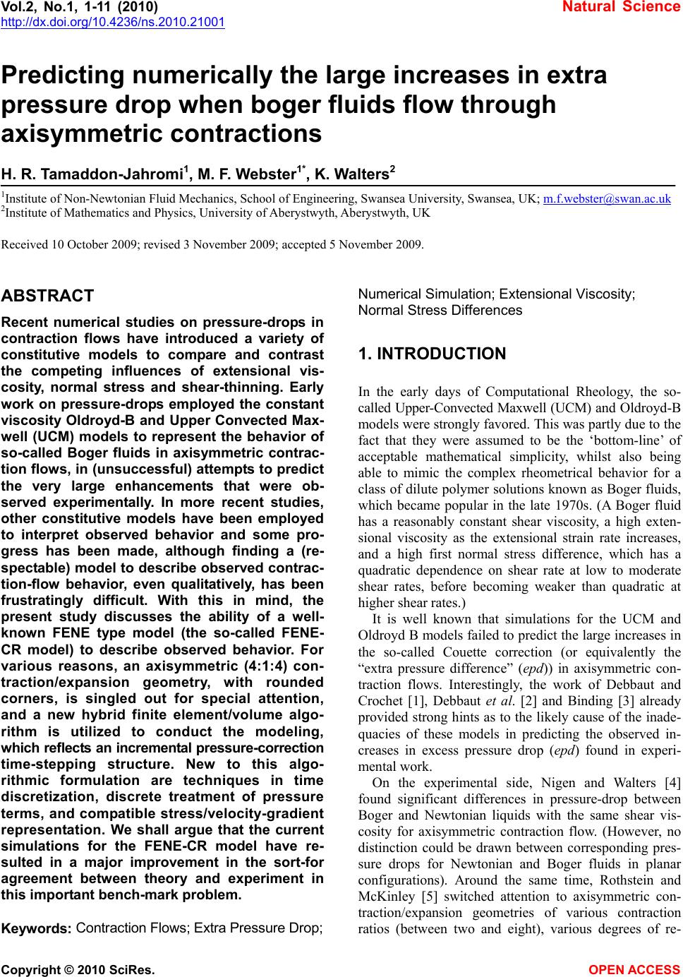Vol.2, No.1, 1-11 (2010) Natural Science
http://dx.doi.org/10.4236/ns.2010.21001
Predicting numerically the large increases in extra
pressure drop when boger fluids flow through
axisymmetric contractions
H. R. Tamaddon-Jahromi1, M. F. Webster1*, K. Walters2
1Institute of Non-Newtonian Fluid Mechanics, School of Engineering, Swansea University, Swansea, UK;
2Institute of Mathematics and Physics, University of Aberystwyth, Aberystwyth, UK
Received 10 October 2009; revised 3 November 2009; accepted 5 November 2009.
ABSTRACT
Recent numerical studies on pressure-drops in
contraction flows have introduced a variety of
constitutive models to compare and contrast
the competing influences of extensional vis-
cosity, normal stress and shear-thinning. Early
work on pressure-drops employed the constant
viscosity Oldroyd-B and Upper Convected Max-
well (UCM) models to represent the behavior of
so-called Boger fluids in axisymmetric contrac-
tion flows, in (unsuccessful) attempts to predict
the very large enhancements that were ob-
served experimentally. In more recent studies,
other constitutive models have been employed
to interpret observed behavior and some pro-
gress has been made, although finding a (re-
spectable) model to describe observed contrac-
tion-flow behavior, even qualitatively, has been
frustratingly difficult. With this in mind, the
present study discusses the ability of a well-
known FENE type model (the so-called FENE-
CR model) to describe observed behavior. For
various reasons, an axisymmetric (4:1:4) con-
traction/expansion geometry, with rounded
corners, is singled out for special attention,
and a new hybrid finite element/volume algo-
rithm is utilized to conduct the modeling,
which reflects an incremental pressure-correction
time-stepping structure. New to this algo-
rithmic formulation are techniques in time
discretization, discrete treatment of pressure
terms, and compatible stress/velocity-gradient
representation. We shall argue that the current
simulations for the FENE-CR model have re-
sulted in a major improvement in the sort-for
agreement between theory and experiment in
this important bench-mark problem.
Keywords: Contraction Flows; Extra Pressure Drop;
Numerical Simulation; Extensional Viscosity;
Normal Stress Differences
1. INTRODUCTION
In the early days of Computational Rheology, the so-
called Upper-Convected Maxwell (UCM) and Oldroyd-B
models were strongly favored. This was partly due to the
fact that they were assumed to be the ‘bottom-line’ of
acceptable mathematical simplicity, whilst also being
able to mimic the complex rheometrical behavior for a
class of dilute polymer solutions known as Boger fluids,
which became popular in the late 1970s. (A Boger fluid
has a reasonably constant shear viscosity, a high exten-
sional viscosity as the extensional strain rate increases,
and a high first normal stress difference, which has a
quadratic dependence on shear rate at low to moderate
shear rates, before becoming weaker than quadratic at
higher shear rates.)
It is well known that simulations for the UCM and
Oldroyd B models failed to predict the large increases in
the so-called Couette correction (or equivalently the
“extra pressure difference” (epd)) in axisymmetric con-
traction flows. Interestingly, the work of Debbaut and
Crochet [1], Debbaut et al. [2] and Binding [3] already
provided strong hints as to the likely cause of the inade-
quacies of these models in predicting the observed in-
creases in excess pressure drop (epd) found in experi-
mental work.
On the experimental side, Nigen and Walters [4]
found significant differences in pressure-drop between
Boger and Newtonian liquids with the same shear vis-
cosity for axisymmetric contraction flow. (However, no
distinction could be drawn between corresponding pres-
sure drops for Newtonian and Boger fluids in planar
configurations). Around the same time, Rothstein and
McKinley [5] switched attention to axisymmetric con-
traction/expansion geometries of various contraction
ratios (between two and eight), various degrees of re-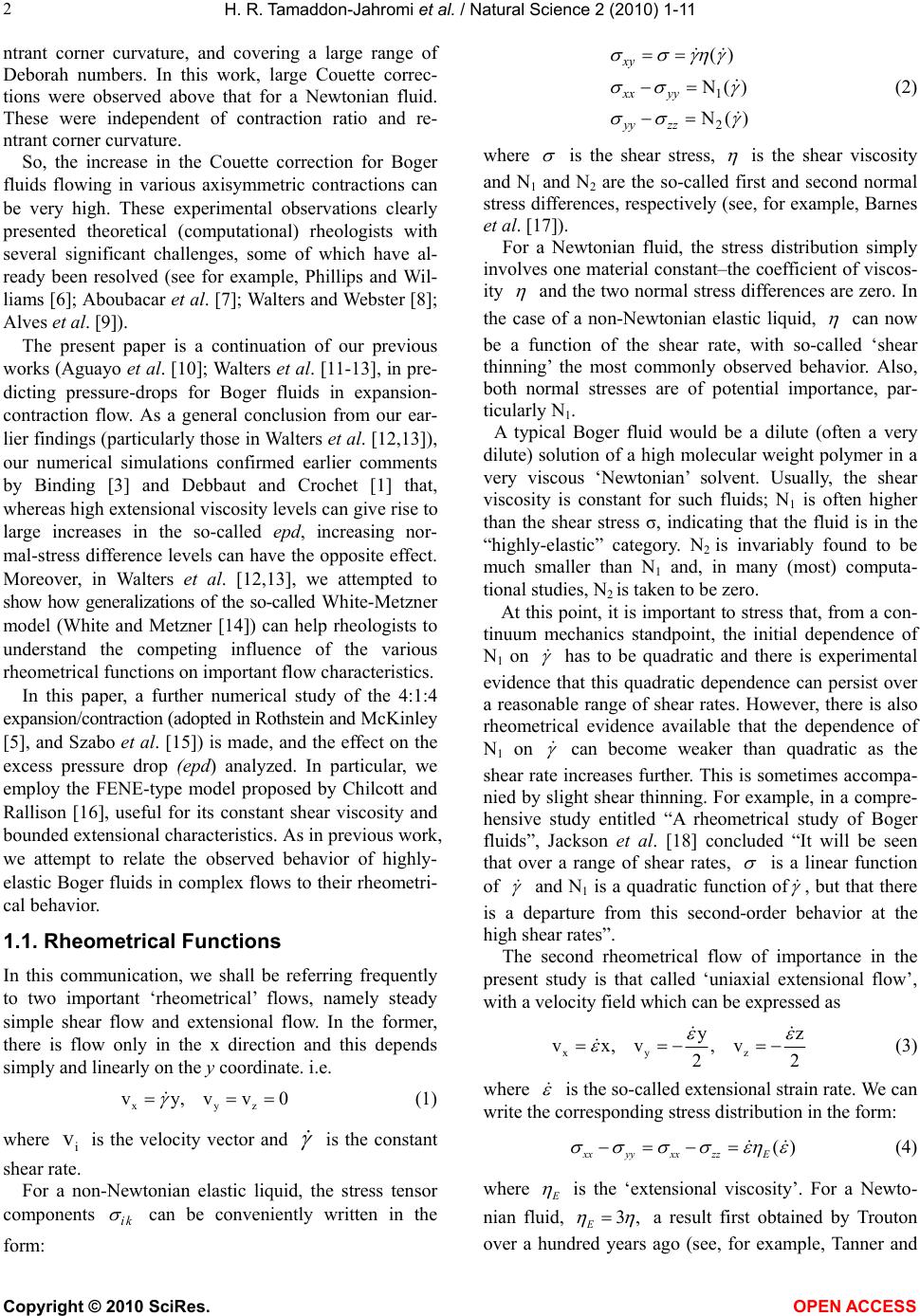

H. R. Tamaddon-Jahromi et al. / Natural Science 2 (2010) 1-11
2
ntrant corner curvature, and covering a large range of
Deborah numbers. In this work, large Couette correc-
tions were observed above that for a Newtonian fluid.
These were independent of contraction ratio and re-
ntrant corner curvature.
So, the increase in the Couette correction for Boger
fluids flowing in various axisymmetric contractions can
be very high. These experimental observations clearly
presented theoretical (computational) rheologists with
several significant challenges, some of which have al-
ready been resolved (see for example, Phillips and Wil-
liams [6]; Aboubacar et al. [7]; Walters and Webster [8];
Alves et al. [9]).
The present paper is a continuation of our previous
works (Aguayo et al. [10]; Walters et al. [11-13], in pre-
dicting pressure-drops for Boger fluids in expansion-
contraction flow. As a general conclusion from our ear-
lier findings (particularly those in Walters et al. [12,13]),
our numerical simulations confirmed earlier comments
by Binding [3] and Debbaut and Crochet [1] that,
whereas high extensional viscosity levels can give rise to
large increases in the so-called epd , increasing nor-
mal-stress difference levels can have the opposite effect.
Moreover, in Walters et al. [12,13], we attempted to
show how generalizations of the so-called White-Metzner
model (White and Metzner [14]) can help rheologists to
understand the competing influence of the various
rheometrical functions on important flow characteristics.
In this paper, a further numerical study of the 4:1:4
expansion/contraction (adopted in Rothstein and McKinley
[5], and Szabo et al. [15]) is made, and the effect on the
excess pressure drop (epd) analyzed. In particular, we
employ the FENE-type model proposed by Chilcott and
Rallison [16], useful for its constant shear viscosity and
bounded extensional characteristics. As in previous work,
we attempt to relate the observed behavior of highly-
elastic Boger fluids in complex flows to their rheometri-
cal behavior.
1.1. Rheometrical Functions
In this communication, we shall be referring frequently
to two important ‘rheometrical’ flows, namely steady
simple shear flow and extensional flow. In the former,
there is flow only in the x direction and this depends
simply and linearly on the y coordinate. i.e.
xyz
vy,vv0


 (1)
where i v is the velocity vector and 

is the constant
shear rate.
For a non-Newtonian elastic liquid, the stress tensor
components ik

can be conveniently written in the
form:
1
2
()
N
()
N
()
xy
xx yy
yy zz












(2)
where

is the shear stress,

is the shear viscosity
and N1 and N2 are the so-called first and second normal
stress differences, respectively (see, for example, Barnes
et al. [17]).
For a Newtonian fluid, the stress distribution simply
involves one material constant–the coefficient of viscos-
ity

and the two normal stress differences are zero. In
the case of a non-Newtonian elastic liquid,

can now
be a function of the shear rate, with so-called ‘shear
thinning’ the most commonly observed behavior. Also,
both normal stresses are of potential importance, par-
ticularly N1.
A typical Boger fluid would be a dilute (often a very
dilute) solution of a high molecular weight polymer in a
very viscous ‘Newtonian’ solvent. Usually, the shear
viscosity is constant for such fluids; N1 is often higher
than the shear stress σ, indicating that the fluid is in the
“highly-elastic” category. N2 is invariably found to be
much smaller than N1 and, in many (most) computa-
tional studies, N2 is taken to be zero.
At this point, it is important to stress that, from a con-
tinuum mechanics standpoint, the initial dependence of
N1 on

 has to be quadratic and there is experimental
evidence that this quadratic dependence can persist over
a reasonable range of shear rates. However, there is also
rheometrical evidence available that the dependence of
N1 on

 can become weaker than quadratic as the
shear rate increases further. This is sometimes accompa-
nied by slight shear thinning. For example, in a compre-
hensive study entitled “A rheometrical study of Boger
fluids”, Jackson et al. [18] concluded “It will be seen
that over a range of shear rates,

is a linear function
of

 and N1 is a quadratic function of

, but that there
is a departure from this second-order behavior at the
high shear rates”.
The second rheometrical flow of importance in the
present study is that called ‘uniaxial extensional flow’,
with a velocity field which can be expressed as
xy z
yz
vx,v ,v
22


 

 (3)
where

 is the so-called extensional strain rate. We can
write the corresponding stress distribution in the form:
()
xxyyxx zzE







(4)
where
E

is the ‘extensional viscosity’. For a Newto-
nian fluid, 3,
E


a result first obtained by Trouton
over a hundred years ago (see, for example, Tanner and

H. R. Tamaddon-Jahromi et al. / Natural Science 2 (2010) 1-11
3
3
R
u
R
u
/4
Walters [19]). For this reason, the ratio between the two
viscosities is called the ‘Trouton ratio TR’, and this
clearly takes the value 3 for a Newtonian fluid. For a
non-Newtonian elastic fluid, TR can be significantly
higher than 3, with ‘orders of magnitude’ increases not
uncommon.
From the above discussion and the relevant literature,
we can associate the following rheometrical behavior
with Boger fluids:
1) A reasonably constant shear viscosity

.
2) A potentially high extensional viscosity
E

as the
extensional strain rate increases.
3) A high first normal stress difference N1, which has
a quadratic shear rate dependence on

, at least for small
to moderate shear rates.
4) A second normal stress difference N2 which is
negative and at most one tenth of the magnitude of N1. It
is often taken as zero in computational studies.
Clearly, any constitutive model that we use to describe
Boger fluids has to satisfy (1)-(4), at least in a semi-
quantitative sense.
2. THE CONTRACTION/EXPANSION
PROBLEM
In conventional contraction flow, liquids are forced
through a contraction under a pressure gradient. At spe-
cific locations on the walls, upstream and downstream of
the contraction, pressure measurements are made. These
locations must be far enough away from the contraction
for the flows to be deemed to be unaffected by the con-
traction, i.e. we may consider the flows to be ‘fully de-
veloped’ and ‘Poiseuille like’ at the pressure-measurement
stations.
In contraction flows, there is often significant interest
in the kinematics of the flow structure, particularly the
vortices which provide computational rheologists with
significant challenges (see, for example, Walters and
Webster [8]). However, in the present work, we shall
confine attention to the dynamics of the flow, which is
often studied through the so-called Couette correction C,
defined by


w
––/
u u d d
C p pL pL 2    (5)
Here, p is the total pressure difference between the
inlet and outlet transducers, u p

is the fully-developed
pressure gradient in the upstream section, d p is the
fully-developed pressure gradient in the downstream
section, u
L and d L are their respective lengths, w

is the fully-developed wall shear stress in the down-
stream channel.
The Couette correction C is usually plotted as a func-
tion of the Deborah number
De= w


 (6)

is a characteristic relaxation time and w

 is the
shear-rate at the downstream wall.
In this paper, the Deborah number is defined as De=
avg


, where avg

 is the average shear-rate in the con-
striction zone.
An alternative measure of ‘resistance to flow’ is the
so-called Excess Pressure Drop (epd), defined by Bind-
ing et al. [20].



*B
N
fd
fd
pp
ppp

, fdu u d d ppL+ pL

 (7)
In this form, p* can be equated to the ratio of Couette
corrections for constant-viscosity Boger and Newtonian
fluids, with corresponding wall shear stress.
The subscripts N and B represent the corresponding
Newtonian and Boger fluid values, respectively, when
these are applicable.
In our recent computational work on contraction flows
(Walters et al. [11-13,21]), we decided to concentrate on
the related contraction-expansion (4:1:4) geometry, with
rounded corners (see Figure 1).
We did this for a number of different reasons. For
example:
1) We found the geometry to be far easier to handle in
the computations than the conventional 4:1 geometry
with sharp corners. Pressure differences were an order of
magnitude lower for the 4:1:4 geometry than with 4:1
geometry flows, with shorter downstream distances de-
manded to establish relaxed stress beyond the constric-
tion (see also Szabo et al. [15] for FENE results). We
have certainly been able to reach higher values of the
Deborah number in the simulations. Furthermore, appli-
cation of the basic numerical method was already well
developed in the Swansea research group.
2) Importantly, experimental data for the 4:1:4 ge-
ometry had been supplied by McKinley and his co-
workers (see, for example, Rothstein and McKinley
Figure 1. Schematic diagram of contraction-expansion
geometry.

H. R. Tamaddon-Jahromi et al. / Natural Science 2 (2010) 1-11
4
[5]). These showed the same trends as those already well
known in the conventional 4:1 geometry. Of major im-
portance was the appearance in the Rothstein and
McKinley experiments of substantial increases in the
epd for increasing Deborah numbers in the case of
Boger fluids.
3. CONSTITUTIVE EQUATIONS
We now need to address the question of choosing appro-
priate constitutive equations for the Boger fluids, which
we shall concentrate on in this publication.
Confining attention to incompressible fluids, we can
write the Cauchy stress tensor ik

in the form:
ik ik ik
Tp   (8)
where p is an arbitrary isotropic pressure, ik

the
Kronecker delta, and ik T is the so-called extra-stress
tensor.
Constitutive equations relate the extra-stress tensor
ik
T to a suitable kinematic variable such as the rate-
of-strain tensorik d. For two specific but very different
reasons, it is often convenient to introduce a so- called
“stress splitting”:
(1)(2 )
ik ikik
TT T (9)
and to write 1()
ik
T as a Newtonian contribution
(1)
1
2
ik ik
Td  (10)
Computational rheologists have often found that the
introduction of the Newtonian component can greatly
assist in the numerical simulation of complex flows, and
experimental rheologists, particularly those working
with Boger fluids, have also found the modification to be
useful. They invariably associate 1

with the solvent
viscosity.
As an example of this stress splitting, consider the
well-known Oldroyd B model, with constitutive equa-
tions are usually expressed in the form:
102
2 ik ik
ik ik
TTd d


 


 (11)
where the triangle denotes the usual upper-convected
time derivative introduced by Oldroyd [22].
It is often convenient to write this equation in the form:
1
0
2  
()
ik ik
Td
22
10
2 


() ()
ik ikik
TT (1-)d
(12)
where 12

 
/
.
For the Boger fluids, which have been used in many
fundamental experimental contraction-flow studies (see,
for example, Boger and Walters [23]), the polymer con-
tribution to the total viscosity is very low. This is domi-
nated by the solvent contribution, so that β is usually in
the range 0.9 to 0.95, or even higher.
The important rheometrical functions for the Oldroyd
B model are given by
0
2
10 1 2
00 22
11
,
N2(1) ,N0,
1
33(1)
12


 



 

 




E
(13)
We see that the Oldroyd B model predicts a constant
shear viscosity0

, a quadratic first normal stress differ-
ence N1, a zero second normal stress difference N2, and a
potentially high extensional viscosity

E
. In fact,

E
reaches an infinite value at a finite value of the exten-
sional strain rate

.
As we have indicated, shear thinning is (virtually) ab-
sent in Boger fluids. Furthermore, the uniaxial exten-
sional viscosity levels can be very high indeed. These
factors have been the main reasons for the popularity of
the Oldroyd B model in Computational Rheology studies
for Boger fluids. The relative simplicity of the model has
been another factor of importance.
However, at this point, it needs to be stressed again
that all existing simulations for the Oldroyd B have been
unable to predict the large increases in the Couette cor-
rection found when Boger fluids flow through axisym-
metric contraction/expansion flows (see, for example
Walters et al. [11-13]).
With this in mind, Walters et al. [12,13] introduced
some new constitutive models to help elucidate the
situation. These were in part guided by ideas put forward
by Debbaut and Crochet (see Debbaut and Crochet [1]
and Debbaut et al. [2]). In these papers, use was made of
two rate-of-strain invariants, which we shall conven-
iently refer to as

 and 

in what follows:
23
ddd
,/IIIII II


(14)
Here, d
II and d III are the two nonzero invariants
of the rate of strain tensor ik
d in their usual form:


1tr
2
dd
,detII III
2
dd
(15)
The reason for the choice (14) instead of (15) has been
fully explained by Debbaut and Crochet [1] and Debbaut
et al. [2]. Clearly, the invariant

 reduces to the usual
shear rate in a steady simple shear flow and the invariant

 reduces to the usual extensional strain rate in a uni-
axial extensional flow. Hence, the reason for the notation,
Walters et al. [12,13] introduced four constitutive mod-
els that they defined as A-D, all of which have the struc-
ture introduced in Eqs.8 to 10.

H. R. Tamaddon-Jahromi et al. / Natural Science 2 (2010) 1-11
5
5
Model A is simply the Newtonian fluid with 2()
ik
T
given by
2
0
21  
()
ik ik
T(-)d
(16)
Model D is the Oldroyd B model we have already in-
troduced in Eqs.11 and 12 with rheometrical functions
given in Eq.13.
Models B and C can be seen as extensions of the mod-
els GNM1 and UCM1 in the Debbaut et al. [2] papers. B
is an inelastic model with 1()
ik
T given as in Eq.12 and

0
2
2
11
21
12






() ik
ik
()d
T()
(17)
The rheometrical functions for model B are
0
1
00 22
11
N0
1
331 12

 




 




E
,
()
,
(18)
i. e. the same

and

E
as the Oldroyd B model, but
with N1=0.
Model C has viscoelastic properties with 1() ik
T given
as in Eq.12 and

0
22
1
2
11
1
2,
12 


 





 
() ()
ik ikik
()
TT (,)d
(,)( )
(19)
In this case, the rheometrical functions are
0
10
0
2
12
N21β
3
N0
E
(),
.
,
,




 




(20)
This time it is

and N1 that match the expressions
for the Oldroyd B model, but

E
now has the Newto-
nian expression.
Model C can be viewed as a “Generalized White-
Metzner model” (see, for example Walters et al. [12]).
The benefit of having the four A-D models available
was that it allowed us the luxury of the following com-
parisons:
1) A comparison of the simulations for models A and
B provided an indication of the effect of extensional
viscosity on flow characteristics, since 0

  and N1=
0 for both models.
2) A comparison of the simulations for models A and
C provided an indication of the effect of “normal
stresses” on flow characteristics, with a “Newtonian”
extensional viscosity in both.
3) A comparison of the simulations for models B and
C provided an indication of the relative strengths of
normal stress and extensional viscosity effects on flow
characteristics.
4) A comparison of the simulations for models C and D
(i.e. the Oldroyd B model) highlighted further the effect of
a high extensional viscosity in the case of elastic liquids.
5) Lastly, a comparison of the simulations for models
B and D highlighted further the normal stress effect,
keeping in mind however that, in this comparison, model
B is inelastic and model D is viscoelastic.
We felt that numerical simulations for the four consti-
tutive models (A-D) could throw considerable light on
the influences of the various rheometrical functions on
flow characteristics.
We show in Figure 2 simulations for the contrac-
tion/expansion geometry provided by Walters et al.
[12,13]. We summarize their findings here, as these have
been fundamental and serve as a basis for the present
study, where a number of additional factors are taken
into account.
The respective simulations of Figure 2 for the four
constitutive models (A-D) demonstrate the influence of
the various rheometrical functions on excess pressure
drop (epd) read against increasing deformation rate (De).
A comparison of models A to B shows the increasing
effect that extensional-viscosity alone has on epd, as
both models support vanishing N1. Alternatively, under
constant extensional viscosity, a comparison of models A
to C indicates that the increasing influence of normal
stress difference can give rise to the opposite effect, that
is a decrease in epd (as suggested in Binding [3]).
3.1. Comparison of Results for Models B and D
Taking this comparison one step further we may contrast
the epd results for model B with those for model D
(Oldroyd B). Here, we note that the Oldroyd B model
reflects the same extensional viscosity as model B (an
example of extreme strain-hardening), but with a
non-zero normal stress difference of quadratic variation
in shear rate (so, N1≠0). Model D is often used to ap-
proximate experimental results for Boger fluids, due to
its constant shear viscosity and strain-hardening proper-
ties. Consistent with the above, the results again demon-
strate a decline in epd from model B to model D, this
being associated with the associated rise in N1. We note
in addition, that there is the usual upper limit on De at-
tainable in the simulations for model D (attributed to the
unbounded nature of ηe). Here, there is a slight dip in
epd before reaching the limiting value at the Newtonian
reference line (for this level of solvent fraction, 0.9),
which lies disappointingly short of the large positive epd
experimental expectations reported for Boger fluids
(Nigen and Walters [4]; Rothstein and McKinley [5]).

H. R. Tamaddon-Jahromi et al. / Natural Science 2 (2010) 1-11
6

N1
10
-3
10
-2
10
-1
10
0
10
1
10
2
10
3
10
4
10
5
10
6
10
-4
10
-3
10
-2
10
-1
10
0
10
1
10
2
10
3
10
4
10
5
[1] Oldroyd-B
[2] FENE-CR,L=100
[3] FENE-CR,L=50
[4] FENE-CR,L=40
[5] FENE-CR,L=30
[6] FENE-CR,L=20
[7] FENE-CR,L=10
[8] FENE-CR,L=5
[9] FENE-CR,L=3

[6]
[2]
[1]
[9]
[1]
[8]
[6]
[9]
Figure 2. Normalized pressure drop (epd) vs. De(=avg

)
for models A-D (cf. Walters et al. [12,13]), β=0.9.
3.2. Comparison of Results for Models C and D
Following this line of study, a direct comparison of epd
results for models C and D, both of which share the same
quadratic N1 behavior, represents the effects of extensional
viscosity alone (recall that model C bears a constant exten-
sional viscosity). Here, once again, we discern an increase
in epd from model C to that for model D.
Clearly, the simulations for models A-D contained in
Figure 2 provide insights into the possibility of provid-
ing numerical simulations which match the experimental
data, at least in a semi-quantitative sense. However, we
still lack definitive evidence that simulations for a (re-
spectable) constitutive equation, which would have gen-
eral acceptance, can provide the required agreement be-
tween experiment and theory. Hence the reason and mo-
tivation for the present work.
We require a model that leads to a constant shear vis-
cosity and possesses other rheometrical features of rele-
vance to Boger-type fluids (also, vanishing N2, see
Chilcott and Rallison [16]). For this reason, we have
alighted on the so-called FENE-CR (Finite Extendible
Nonlinear Elasticity-Chilcott and Rallison [16]) model,
which we shall conveniently refer to as model E. This
has the following constitutive equations:
(1)(2 )
ik ikik
TT T
(1)
1
2
ik ik
Td  (21)
 
(2)
1
1
ik
f
(Tr(A))AI
T  

where the stress is expressed through a conformation
transformation (A) as
10f(Tr(A))AAf(Tr(A))I

   (22)
The stretch function
f
(Tr( A)) depends on L (the
so-called extensibility parameter), and is given by:
2
1
f(Tr(A))= 1-Tr(A)/ L (23)
In this equation, ()TrA is the trace operator and L
essentially measures the size of the polymer molecule in
relation to its equilibrium size. I is the identity tensor.
The associated rheometrical functions are given by
0
2
01
12
2
00
222
11
2(1 )
N,N0
33(1) 2
e
f
f
ff



















(24)
where
f
=f(Tr(A))
is defined in Eq.23.
The rheometrical response of the FENE-CR model is
displayed in Figures 3 and 4. The model predicts a con-
stant shear viscosity, but the first normal stress differ-
ence (N1) is weaker than the strong quadratic form ex-
hibited by the Oldroyd-B model. One notes, however,
that predictions for large values of the extensibility pa-
rameter (L>100) asymptote to Oldroyd-B behavior in N1
and ηe. For small values of L (e.g. L=3), significant de-
parture in N1 is observed from an Oldroyd-B response. A
monotonic decline in N1 is apparent with decreasing L
(Figure 3).
The extensional viscosity behavior of the FENE- CR
model for low extensional strain-rates up to 0.5 is prac-
tically identical to that for the Oldroyd-B model. Beyond
this station, the extensional viscosity for the FENE-CR
model is capped, with the limiting level of the exten-
sional viscosity plateau depending on the elevation of L.
This is illustrated in Figure 4, where the trend in exten-
sional viscosity for the FENE-CR model is almost flat
for L=3. There is advancing earlier departure from
Oldroyd-B trends with appropriate choices of L.
Figure 3. Normal stress data for model E (FENE-CR),
increasing L.

H. R. Tamaddon-Jahromi et al. / Natural Science 2 (2010) 1-11
7
7
Figure 4. Extensional viscosity data for model E (FENE-CR), increasing L.
These are some of the reasons why we thought that a
numerical study of model E in contraction/expansion
flow would be useful.
4. NUMERICAL BACKGROUND
4.1. Hybrid Finite Element/Finite Volume
Scheme
The hybrid finite element/volume scheme employed is a
semi-implicit, time-splitting, fractional staged formula-
tion, which draws upon finite element discretization for
velocity-pressure approximation and finite volume for
stress (see Webster et al. [24], Matallah et al. [25]). Un-
der the fe construction, a two-step Lax-Wendroff scheme
is employed, a Taylor-Galerkin variant (Donea [26],
Zienkiewicz [27]), alongside an incremental pressure-
correction procedure (with 0θ11). For solenoidal con-
ditions and with a forward time increment factor θ2=0.5,
this pressure-correction scheme attracts second-order
temporal accuracy, with its incremental form (θ1>0)
proving superior in uniform temporal error bound at-
tainment over its non-incremental counterpart (θ1=0).
The three-stage structure can be conveniently expressed
(Wapperom and Webster [28]) in semi-discrete repre-
sentation on the single time step [tn; tn+1], with starting
values [un; τn, pn, pn-1], via:


1
2 1
1
21
2Re
12()
2
nn
nn
nnnnn
G
dd
Stage a: uupppF
t



 






 
 


1
21
2n
nnT
We
fIfuLL
t



 






*
(1/ 2)(1/ 2)
* 1
1
Re
12()
2
n
nn
nnnn
G
dd
Stage b: uupppF
t





 


 
 

1
12
1
n
nn T
We
f IfuLL
t

 


 
21 *
2
Re
2nn
Stage : ppu
t


 
 
1* 1
2
2Re
3: nnn Stage uupp
t

 

 (25)
Here, Lu, and the Reynolds number is defined
according to convention as 0 Re /U



 , where ρ is the
fluid density and U,  are characteristic velocity and
length scale of the flow, and 0

is the total viscosity.
Galerkin discretization may be applied to the em-
bedded Stokesian system components; the momentum
equation at Stage 1, the pressure-correction equation at
Stage 2 and the incompressibility satisfaction con-
straint at Stage 3 (to ensure higher order precision). An


e
10
-3
10
-2
10
-1
10
0
10
1
10
2
10
3
10
4
10
5
10
6
10
-1
10
0
10
1
10
2
10
3
10
4
10
5
[1] Oldroyd-B
[2] L =100
[3] L =50
[4] L =40
[5] L =30
[6] L =20
[7] L =10
[8] L =5
[9] L=3
.
[1]
[2]
[3]
[4]
[5]
[6]
[7]
[8]
[9]
1
2
3
1
2
[1] Oldroyd-B
[2] L = 100
[3] L =50
[4] L =40
[5] L =30
[6] L =20
[7] L =10
[8] L =5
[9] L=3
[1] [2] [3]
[4]
[5]
[6]
[7]
[8]
[9]

H. R. Tamaddon-Jahromi et al. / Natural Science 2 (2010) 1-11
8
fe-cell
nodes()
fv-cell
midsidenodes (u, )
vertex nodes (p, u,)
l
(mdc)
T
1
T
2
T
3
T
4
T
5
T
6

i
T
j
l
k
j
k
element-y-element Jacobi solution procedure is util-
ized at Stage 1 (momentum) and Stage 3 for the re-
sulting Galerkin-type Mass matrix-vector equations.
This is an efficient and accuracy technique, requiring
only a handful of iterations and a mixture of exact and
numerical integration rules. This offers a space-time
trade-off, so that huge problems may be accommo-
dated (3D, multiple relaxation times, multi-scale). At
Stage 2, a direct Choleski decomposition is required,
necessitating only a single matrix reduction phase
necessary at the outset. Then, semi-implicitness is in-
troduced at Stages 1a,b on pressure and diffusive terms
to enhance stability in the strongly viscous regime.
Note that, pressure temporal increments invoke multi-
step reference across three successive time levels [tn-1,
tn, tn+1].
4.2. Finite Volume Fluctuation Distribution
Scheme
The theory may be exposed by first expressing the extra-
stress equation in non-conservative form, with flux
(,u.R) and absorbing remaining terms under the
source (Q), one may obtain:
t


RQ (26)
Then, cell-vertex fv-schemes are applied to this
equation utilizing fluctuation distribution as the up-
winding technique, to distribute control volume re-
siduals and furnish nodal solution updates (Wapperom
and Webster [29]). We consider each scalar stress
component, ,

acting on an arbitrary volume
l
l
 
, whose variation is controlled through
corresponding components of fluctuation of the flux (R)
and the source term (Q),
lll
dRdQd
t
 

(27)
Flux and source variations are evaluated over each fi-
nite volume triangle (Ωl), and are subsequently allocated
by the chosen cell-vertex distribution scheme to its three
vertices. In this manner, by summing all contributions
from its control volume Ωl, the nodal update is obtained
composed of all fv-triangles surrounding node (l). The
flux and source residuals may be evaluated over two
separate control volumes associated with a given node (l)
within the fv-cell T. This generates a contribution gov-
erned over the fv-triangle T, (RT, QT), and that subtended
over the median-dual-cell zone, (Rmdc, Qmdc). For reasons
of temporal accuracy, this procedure demands appropri-
ate area-weighting to maintain consistency, with exten-
sion to time-terms likewise. A generalized fv-nodal up-
date equation may be expressed per stress component,
by separate treatment of individual time derivative, flux
and source terms, and integrating over associated control
volumes, yielding,


1
1
1
ll
ll
n
TT
l
Tl TTl
TMDC
TT MDC
TlT l
TMDC
ˆ
t
bb





 






 
 
(28)
where (),
T
TT
bRQ 

l
MDC
lMDCMDC
bRQ ,
T

is the area of the fv-triangle T, and T
l
ˆ

is the
area of its median-dual-cell (MDC). The weighting pa-
rameter, 01
T



, directs the balance taken between
the contributions from the median-dual-cell and the fv-
triangle T. The discrete stencil of Eq.27 identifies
fluctuation distribution and median dual cell contribu-
tions, area weighting and upwinding factors (T
l

-
scheme dependent). The interconnectivity of the
fv-triangular cells (i
T) surrounding the sample node (l),
the blue-shaded zone of mdc, the parent triangular fe-cell,
and the fluctuation distribution (fv-upwinding) parame-
ters (T
i

), for i=l, j, k on each fv-cell, are all features
illustrated in Figure 5.
5. NUMERICAL PREDICTIONS
As we have indicated, the benchmark problem we wish
to address is that of flow within a 4:1:4 axisymmetric
rounded-corner contractions (Figure 1). In this study,
creeping flow is assumed (Re≈10-2). We concentrate
again on the epd defined in Eq.7, rather than the Couette
correction, and we restrict attention to β=0.9 and 1/9.
Figure 5. Spatial discretisation: fe-cell with four fv-subcells
and fv control volume for node l with median-dual-cell
(shaded).

H. R. Tamaddon-Jahromi et al. / Natural Science 2 (2010) 1-11
9
9
5.1. Effect of Normal Stress (N1) and
Extensional Viscosity (ηe) on epd
Comparison of Results for Models D
(Oldroyd B) and E (FENE-CR)
The important new simulation results are contained in
Figures 6-10, in which we see epd data for both the
Oldroyd B model and variants of the FENE-CR model.
It is clear that our simulations for the Oldroyd B
model reach a limit at Decrit=5.1 (see Figure 8), evi-
dently due to unbounded ηe and over-strong N1; and we
have been unable to reach higher Deborah numbers.
Hence, unfortunately, for β=0.9, we have been unable to
break through the epd=1.0 barrier (epd=0.999792 at De
=5.1), whilst for β=0.95, a positive value of ep d is ob-
tained. We have previously confirmed such results
through spatial resolution with three different meshes;
see Aguayo et al. [10].
This state of affairs may be contrasted with that for
the FENE-CR model, which is bounded in extension and
has a weakened N1 behavior (see Figure 3). As above,
we can anticipate a lowering of epd values due to ηe
damping and an elevation due to N1 damping. There
must clearly be a trade-off between these two factors;
but at least we have been able to reach relatively high
values of De in the FENE-CR simulations. Over the
range of De values covered in Figure 6, we see an in-
crease in epd values for L=5 of approximately 15% at
De=10, and in the extended range covered in Figure 7
this rises to approximately 28%. Here, in the several
decades beyond De=10, ηe is noted to approach its limit-
ing upper plateau, so that continued further increase in
epd can only be attributed to continual weakening of N1
from its quadratic form. So, from a qualitative standpoint,
much progress has been made, although it must be ad-
mitted that we are still some way from the extravagant
increases in epd found in some of the experiments on
Boger fluids.
In Aguayo et al. [10] and for steady flow, it was
shown that epd in these 4:1:4 flows can only be influ-
enced by shear and extensional contributions within
the geometry constriction region excluding the shear
upstream-downstream zones. Below we note just how
important the shear component (N1) can be in this
mixed flow region (best interpreted in a Lagrangian
sense). One can attempt to segregate the various com-
peting factors through comparison with pairings of
L-parameter epd data. For example, comparing data in
Figure 6 for lower values of L={3,5} and the defor-
mation rate range 0≤De≤3.33, one can observe the
elevating effect from L=5 to L=3 on epd of gradually
weakening N1 (which is the dominant influence in this
range). This outcome cannot be attributed to the de-
clining influence of ηe (see Figure 4), as if anything,
this would have a counter-effect on epd. Subsequently,
in the range De>3.33, extensional viscosity effects
begin to dominate, as observed in the consistently lar-
ger epd-values for L=5; leading to upper limits at
De=10 (above the Newtonian reference level) some
three times larger with L=5 (epd=1.15) than for L=3
(epd=1.05). Note, that the transition zone-point (De≈
3.33) is highlighted in Figure 6, where N1 and ηe in-
fluential dominance switches over.
The same argument for domination of N1-weakening/
ηe-strengthening holds true for the L={3,10} and {5,10}
data; with shifts in the transition point to De≈7 for
L={3,10} and to De≈8.5 for L={5,10}. For L=10 data
and in contrast to Oldroyd-B epd-data in Figure 8,
weakening N1 behavior for the FENE-CR model ele-
vates epd up to the intersection/transition point (De≈2.5).
Over 2.5≤De≤5, the stronger ηe of the Oldroyd model
increasing prevails, so that larger ηe gives larger epd, a
trend anticipated to continue as De rises (nb. Decrit=5.1,
Oldroyd-B). In contrast, the F extension/weakening of
N1) achieves a Decrit=9 at which the increase in epd ad-
vances to around 18%.
Considering larger values of the extensibility parameter
(L≥40, with larger ηe plateaux) in Figure 9, all FENE-
CR epd results are now qualitatively similar to those-
for the Oldroyd-B model, with transition point (gov-
Figure 6. Normalised pressure-drop (epd) vs De(= avg


)
for model E (FENE-CR, L=3, 5), β=0.9.
Figure 7. Normalised pressure-drop (epd) vs De(= avg


)
for model E (FENE-CR, L=5), β=0.9.
1
5
%
5%
28%

H. R. Tamaddon-Jahromi et al. / Natural Science 2 (2010) 1-11
10
Figure 8. Normalised pressure-drop (epd) vs De(= avg 
) for
model E (FENE-CR, L=10) and model D (Oldroyd-B), β=0.9.
erning dominance) shifting to the lower value De≈2.
Here, relative to the Oldroyd-B epd-data, there is
slight elevation of epd for De≤2 (N1-dominating) and
slight suppression of epd for De>2 (ηe-dominating).
For completeness, we include simulations for a (lower)
value of solvent fraction β, namely β=1/9. In the early
days of Computational Rheology, this value was favored,
the reasoning being associated with the realization that,
for some models such as the so-called Corotational
Oldroyd Model, higher values of β would lead to a non-
monotonic shear-stress/shear-rate response. It must be
emphasized that such a restriction is not relevant to the
Oldroyd B model and is certainly not appropriate for
Boger fluids, where we have argued that β=0.9 (and
higher) is more realistic. However, to enable a compari-
son to be made with some earlier studies, we include in
Figure 10 simulations for β=1/9 (low solvent fraction,
high polymeric contribution).
These simulations are in general agreement with those
of Szabo et al. [15], who also noted epd enhancement for
L=5, β=1/9, accompanied with the explanation that…“a
particular value of L=5 needed less stretch to achieve
full extension” and a sink flow (pure extension) analysis
to identify pressure drop upturn and vortex behavior. We
observe, by inspection across L-values at fixed De for
β=1/9, that it is the dominating influence of N1 that is
clearly apparent with no transition points to ηe domina-
tion. Interpreted at any particular De, as L rises, N1 in-
creases in strength and epd declines monotonically. Un-
der such conditions, ηe -plateaux also rise and so would
be anticipated to only contribute to epd-enhancement.
Hence, the suppressive influence of N1-rise must counter
this to generate decline in epd.
Viewed at each L-value and rising De, earlier argu-
ments reapply governing the competing influences upon
epd. This yields a rise of around 13% in epd for L=3 at
De=4. In contrast, the position is adjusted accordingly
for L=5 and L=10 data, with gradual strengthening of
N1-influence. Hence, for L=10, one detects a local
minimum at De=3, beyond which there is an ‘upturn’.
Figure 9. Normalized pressure-drop (epd) vs De (= avg


)
for model E (FENE-CR, L=40,50,100) and model D
(Oldroyd-B), β=0.9.
Figure. 10. Normalised pressure-drop (epd) vs De(= avg


)
for model E (FENE-CR, L=3-50) and model D (Oldroyd-B),
β=1/9.
However, the overall lowering of epd-level at L=10 is
such that there is insufficient recovery for De>3 to cross
the Newtonian reference line, as occurs with L=3 and
L=5 epd-data.
6. CONCLUSIONS
The current work has covered the numerical prediction
of the excess pressure drop (epd) for the flow of FENE-
CR fluids through a 4:1:4 contraction/expansion geome-
try with rounded corners. A detailed study of epd and
associated parameters has revealed some interesting and
provocative results.
Unlike the inadequacies of the Oldroyd B model in
observing the experimentally observed increases in epd,
various forms of the FENE CR model, possessing first
normal stress differences weaker than the strong quad-
ratic form of the Oldroyd B model, are capable of pre-
dicting enhanced epd.
We are encouraged by the fact that we have been able
to reach epd elevations of nearly 30%, and this is clearly
a step in the right direction. However, this is still some
way short of some of the large epd-levels found experi-
18%
13%

H. R. Tamaddon-Jahromi et al. / Natural Science 2 (2010) 1-11
11
11
mentally for Boger fluids. In addition, we are a little
concerned that the various parameters in the FENE-CR
model, such as L, are not physically representative at the
molecular level, (something which is of course well docu-
mented in the literature), and, more importantly, that they
have needed to be chosen so precisely in the present work
to obtain the desired effect. This suggests some form of
dynamic and locally rate-responsive scale would be
more appropriate, as commended through the FENE-
Adaptive- Length-Scale (ALS) model (Ghosh et al. [30]).
So, there are still questions to be answered, but at least
some progress has been (and is being) made! In the fu-
ture, this work will be extended to analyze the additional
adjustment when shear-thinning properties are intro-
duced; and also alternative flow scenarios where energy
related issues are pertinent, such as drag characteristics
in flow past a sphere.
REFERENCES
[1] Debbaut, B. and Crochet, M.J. (1988) Extensional effects
in complex flows. J Non-Newton Fluid Mech, 30, 169-184.
[2] Debbaut, B., Crochet, M.J., Barnes, H.A. and Walters, K.
(1988) Extensional effects in inelastic liquids. Xth Inter.
Congress on Rheology, Sydney, 291-293.
[3] Binding, D.M. (1991) Further considerations of axisym-
metric contraction flows. J Non-Newton Fluid Mech, 41,
27-42.
[4] Nigen, S. and Walters, K. (2002) Viscoelastic contraction
flows: comparison of axisymmetric and planar configu-
rations. J Non-Newton Fluid Mech , 102, 343-359.
[5] Rothstein, J.P. and McKinley, G.H. (2001) The axisym-
metric contraction-expansion: The role of extensional
rheology on vortex growth dynamics and the enhanced
pressure drop. J Non-Newton Fluid Mech, 98, 33-63.
[6] Phillips, T.N. and Williams, A.J. (2002) Comparison of
creeping and inertial flow of an Oldroyd B fluid through
planar and axisymmetric contractions. J Non-Newton
Fluid Mech, 108, 25-47.
[7] Aboubacar, M., Matallah, H., Tamaddon-Jahromi, H.R.
and Webster, M.F. (2002) Numerical prediction of exten-
sional flows in contraction geometries: Hybrid finite vol-
ume/element method. J Non-Newton Fluid Mech, 104,
125-164.
[8] Walters, K. and Webster, M.F. (2003) The distinctive
CFD challenges of computational rheology. Inter J for
Numer Meth in Fluids, 43, 577-596.
[9] Alves, M.A., Oliveira, P.J. and Pinho, F.T. (2004) On the
effect of contraction ratio in viscoelastic flow through ab-
rupt contractions. J Non-Newton Fluid Mech, 122, 117-130.
[10] Aguayo, J.P., Tamaddon-Jahromi, H.R. and Webster, M.F.
(2008) Excess pressure-drop estimation in contraction
flows for strain-hardening fluids. J Non-Newton Fluid
Mech, 153, 186-205.
[11] Walters, K., Webster, M.F. and Tamaddon-Jahromi, H.R.
(2009a) The numerical simulation of some contraction
flows of highly elastic liquids and their impact on the
relevance of the Couette correction in extensional rheol-
ogy. Chem Eng Sci, 64, 4632-4639.
[12] Walters, K., Webster, M.F. and Tamaddon-Jahromi, H.R.
(2009b) The White-Metzner model then and now. Pro-
ceedings of the 25th Annual Meeting of the PPS meeting,
Goa, India, 02, 1-14.
[13] Walters, K., Tamaddon-Jahromi, H.R., Webster, M.F.,
Tomé, M.F. and McKee, S. (2010) The competing roles
of extensional viscosity and normal stress differences in
complex flows of elastic liquids. Korean-Australian
Journal (to be published), 2010.
[14] White, J.L. and Metzner, A.B. (1963) Development of
constitutive equations for polymeric melts and solutions.
J Appl Polym Sci, 7, 1867-1889.
[15] Szabo, P., Rallison, J.M. and Hinch, E.J. (1997) Start-up
of flow of a FENE-fluid through 4:1:4 constrictions in a
tube. J Non-Newton Fluid Mech, 72, 73-86.
[16] Chilcott, M.D. and Rallison, J.M. (1988) Creeping flow
of dilute polymer solutions past cylinders and spheres. J
Non-Newton Fluid Mech, 29, 381-432.
[17] Barnes, H.A., Hutton, J.F. and Walters, K. (1989) An
introduction to rheology. Elsevier, Amsterdam.
[18] Jackson, K.P., Walters, K. and Williams, R.W. (1984) A
rheometrical study of Boger fluids. J Non-Newton Fluid
Mech, 14, 173-188.
[19] Tanner, R.I. and Walters, K. (1998) Rheology: An his-
torical perspective, Elsevier Science & Technology,
Netherlands.
[20] Binding, D.M., Phillips, P.M. and Phillips, T.N. (2006)
Contraction/expansion flows: The pressure drop and re-
lated issues. J Non-Newton Fluid Mech, 137, 31-38.
[21] Walters, K., Webster, M.F. and Tamaddon-Jahromi, H.R.
(2008) Experimental and computational aspects of some
contraction flows of highly elastic liquids and their im-
pact on the relevance of the Couette correction in exten-
sional rheology. Proc. 2nd Southern African Conference
on Rheology (SASOR 2), 1-6.
[22] Oldroyd, J. G. (1950) On the formulation of rheological
equations of state. Proc. Roy .Soc., A200, 523-541.
[23] Boger, D.V. and Walters, K. (1993) Rheological phe-
nomena in focus, Elsevier Science Publishers.
[24] Webster, M.F., Tamaddon-Jahromi, H.R. and Aboubacar,
M. (2005) Time-dependent algorithms for viscoelastic
flow: Finite element/volume schemes. Numer Meth Par
Diff Equ, 21, 272-296.
[25] Matallah, H., Townsend, P. and Webster, M.F. (1998)
Recovery and stress-splitting schemes for viscoelastic
flows. J Non-Newton Fluid Mech, 75, 139-166.
[26] Donea, J. (1984) A Taylor-Galerking method for convective
transport problems. Int J Numer Methods Eng, 20, 101-119.
[27] Zienkiewicz, O.C., Morgan, K, Peraire, J., Vandati, M.
and Löhner R. (1985) Finite elements for compressible
gas flow and similar systems. Seventh International
Conference on Computational Methods of Applied Sci-
ence and Engineering.
[28] Wapperom, P. and Webster, M.F. (1999) Simulation for
viscoelastic flow by a finite volume/element method.
Comput Meth Appl Mech Eng, 180, 281-304.
[29] Wapperom, P. and Webster, M.F. (1998) A second-order
hybrid finite-element/volume method for viscoelastic
flows. J Non-Newton Fluid Mech, 79, 405-431.
[30] Ghosh, I., Lak, Joo Y., McKinley, G.H., Brown, R.A. and
Armstrong, R.C. (2002) A new model for dilute polymer
solutions in flows. J Rheol, 46(5), 1057-1089.