Engineering, 2010, 2, 12-21
doi:10.4236/eng.2010.21002 Published Online January 2010 (http://www.scirp.org/journal/eng/).
Optimum Load Shedding in Power System Strategies with
Voltage Stability Indicators
P. AJAY-D-VIMAL RAJ, M. SUDHAKARAN
Department of Electrical and Electronics Engineering,
Pondicherry Engineering College, Pondicherry, India
Received August 20, 2009; revised September 23, 2009; accepted September 28, 2009
Abstract
An optimal load shedding strategy for power systems with optimum location and quantity of load to be shed
is presented in this paper. The problem of load shedding for avoiding the existence of voltage instability in
power systems is taken as a remedial action during emergency state in transmission and distribution sec-
tor.Optimum location of loads to be shed is found together with their optimum required quantity. L-Indicator
index is in used for this purpose with a modified new technique. Applications to be standard 6 bus
Ward-Hale test system and IEEE – 14 bus system are presented to validate the applicability of the proposed
technique to any system of any size.
Keywords: Load Shedding, Voltage Instability, Power systems, Transmission and Distribution Power system
1. Introduction
The major objective of power systems is to supply elec-
tricity to its customers. During emergency state of the
power system, it may shed partial loads to ensure the
power supply to important loads, as the last resort to
maintain system integrity. Load shedding in bulk power
system has been studied many years [1–6].
In electric power systems heavy loading may lead to
voltage instabilities or collapses or in the extreme to
complete blackouts. One technique of avoiding voltage
instability is to shed some consumer’s loads in Order to
draw the operating point for away from the critical volt-
age value.
Many techniques have been developed [7–13] to mini-
mize the load curtailment without violating the system
security constraints. The emergency state in the power
System with distributed generations has been formulated
the load shedding is solved as an optimization problem
[14]. Ying Lu et al. [15] has proposed a load shedding
scheme, working with various load models, such as sin-
gle-motor model, two-motor model, and composite
model. Armanda et al. [16] have adopted a Distributed
Interruptible Load Shedding (DILS) program instead of
the traditional methodologies based on the separation of
some users and/or entire distribution feeders, according
to programmed plans of emergency. Andrzej Wiszn-
iewski [17] have formulated a new method for estimating
the voltage stability margin, which utilizes local meas-
urements and applied criterion is based on the very defi-
nition of the voltage stability. Zhiping Ding et al. [18]
have developed an expert-system-based load shedding
scheme (LSS) for ship power systems. Emmanuel J.
Thalassinakis et al. [19] have built an efficient computa-
tional methodology that can be used for calculating the
appropriate strategy for load shedding protection in
autonomous power systems.
In this paper a fast method for determining the loca-
tion and quantity of the load to be shed in order to avoid
risk of voltage instability is presented. The method de-
fines clearly the bus where load shedding should make.
A relation between voltage stability indicator changes
and load power to be shed is developed. Using the rela-
tion the amount of load to be shed is determined. An
algorithm has been developed for determining the loca-
tion and quality of load to be shed and tested with tbe
standard 6 buses Ward-Hale test system and IEEE – 14
bus system. The proposed method is valid for any system
of any size at any loading conditions.
2. Mathematical Calculation for Load
Shedding Using Voltage Stability
Indicator- METHOD I
From the indicator proposed in [3] voltage stability indi-

P. AJAY-D-VIMAL RAJ ET AL. 13
cator at bus j can determine by
j
αGi iji
jV
VC
1 B


 (1) αLj
where
: Set of load buses.
L
α
: Set of generator buses.
G
α
: Voltage of generator bus i.
i
V
: Voltage of load bus j.
j
V
: Elements of matrix C determined by
ji
C


C=- (2)

-1
LL
BLG
B 
 

-1
LL
Bis the imaginary part of the matrix

1
LL
Y

LG
B 
 




is the imaginary part of the matrix
LG
Y 


-1
LL
Band are susceptance matrices.
LG
B 


LL
Yand are submatrices for the Y-Bus
matrix.
LG
Y


The indicator at bus j, determined by equation (1) can
be separated into real and imaginary parts :

RI
jj
B,B
αG
ji i
i =1
j
j
CV
B= 1-
V
i
j



(3)
αG
ji i
RI i =1
jj
j
CVδi-δj
B+jB= 1-
V

(4)

j
αG
1i iji
R
jV
δjδicos VC
1B

 
 (5)

αG
ji i
I i=1
j
j
CVsinδi-δj
B= -
V

(6)
δi,δ: voltage angles at buses i and j j
i
V,j
V :voltage magnitudes at buses i and j
The voltage stability indicator at each bus is a function
of voltage angle and magnitude. The real imaginary part
of indicator can be expressed as:


I
1
R
2
B=F δ,V
B=F δ,V
(7)
The partial derivative of Equations (5) and (6) with
respect to voltage angle and magnitude changes can be
determined as:

II
I
RRR
BB
δVΔδ Δδ
ΔBT
ΔVΔV
ΔBBB
δV



 

   

 
   






(8)
Matrix [T] is sensitivity matrix between indicator
changes and voltage angle and magnitude changes
Coefficient of matrix [T] can be determined as


cos
Iji i
J
j
CVi j
B
iV





 ,G
iis


(9)
(S indicates the swing bus)


ji i
I
jR
iαG
j
j
CVcosδi-δj
B=- B-1
δjV
f




(10)
R
jjii
j
BCVsin(δi-δj)
δiV

 (11)
ji i
R
jI
iαG
j
j
CVsin(δi-δj)
BB
δjV






(12)
ji i
II
jj
iαG
2
jj
j
CVsin(δi-δj)
BB
-
VV
V




(13)


ji i
RR
jj
iαG
2
jj
j
CVcosδi-δj
BB
=
VV
V



-1
-

(14)
From conventional Newton-Raphson load flow we
obtain a linear relation between changes in voltage
phases/magnitudes and active/reactive power injections
as:

-1
Δδ ΔP
=j
ΔVΔQ
 
 
 
 (15)
Sub (15) in (8) we get a relationship between real and
imaginary part indicators and injected power as:

I-1
R
ΔBΔP
=T jΔQ
ΔB
 
 
 

(16)
A relationship between changes in indicators at load
bus j and power injections at all load buses can be ob-
tained:
I
j11j12 j
ΔB=S ΔP+S ΔQ (17)
R
j21j22
ΔB=SΔP+S ΔQj (18)

14 P. AJAY-D-VIMAL RAJ ET AL.
The active and reactive loads are not independent; one
cannot shed active load, without curtailing reactive loads.
Usually, a relation between active and reactive load at
bus j can be obtained as follows. Here the load power
factor is assumed to be constant at each load bus.
j
j
j
Q
Pf= P
L
jα
j
j
j
Q
Pf P



jj
QPfP
j
j
j
j
(19)
Sub (19) in (17and18) we get a relationship between
changes of the indicator at bus j and changes in active
power injected at the same bus can be obtained as
I
j11j12j j
ΔB=S ΔP+S PfΔP (20)
R
j21j22j
ΔB=S ΔP+S PfΔP (21)
I
j1
ΔBSΔP (22)
R
j2
ΔBSΔP (23)
where
11112j
S=S+SPf
22122
S=S +S Pf
j
We know

2
I2 R
jj j
ΔB= (ΔB) + ΔB (24)
22 22
j1j2j
ΔB= S ΔP+SΔP (25)
22 2
j12j
ΔB= (S+S)ΔP
s
22
jj12
ΔB=ΔP(S+S) (26)
j
j22
12
ΔB
ΔP
(S +S)
 (27)
jj
ΔQ=PfΔPj (28)
Using Equation (28) reactive power to be shed at bus j
can be obtained if the active power to be shed at bus j is
known.
3. Improved Method for Load Shedding By
Voltage Stability Indicator
There are several methods for improving the voltage
conditions in a power system as suggested in various
articles.
In the improved method, the voltage profile is en-
hanced by determining the location and quantity of load
to be shed, such that voltage instability can be avoided.
This method is based on the indicators of risk of volt-
age instability suggested by P. Kessel and H. Glavitsch
[3]. The improved technique is a modification of the
technique for previous section. It defines clearly the bus
where the load shedding should be made. A relation be-
tween indicator changes and load powers to be shed is
developed here. Using this relation, the amount of load to
be shed is determined, for any operational situation.
4. Mathematical Calculation for Load
Shedding Using Improved Voltage
Stability Indicator- METHOD II
Kessel and Glavitsch [3] have developed a voltage sta-
bility indicator at load bus j
ji i
iαG
j
j
FV
L= 1- V


(29) JαL
where
L
α : Set of load buses.
G
α : Set of generator buses.
i
V : Voltage of generator bus i.
Vj : Voltage of load bus j.

GG GL
LG LL
Y Y
Y= Y Y





 (30)


-1
LL LG
F=-[Y] [Y] (31)
GG
Y, ,,: Elements of system admittance
matrix
LL
YLG YGL Y
A global voltage stability indicator of a power system
is given by L, 0L 1


0: far away from voltage instability point.
1: at voltage instability point.
The indicator at bus j determined by Equation (29) can
be separated into real and imaginary part
RI
jj
(L,L )
jiijiij
RI i αG
jj
j
FV +δ-δ
L+jL= 1-
V



(32)
jiijii j
R i αG
j
j
FVcos +δ-δ
L1-
V



(33)

P. AJAY-D-VIMAL RAJ ET AL. 15
jiijii j
I i αG
j
j
FVsin +δ-δ
L-
V


 (34)
The voltage stability indicator at each bus is a function
of voltage angles and magnitudes. The real and imagi-
nary parts of indicators can be expressed as:

I
1
L=F δ,Vd

(35)

R
2
L=Fδ,V

(36)
The partial derivative of Equations (33) & (34) with
respect to voltage angle and magnitude changes can be
determined as

II
I
RRR
LL
δVΔδ Δδ
ΔLT
ΔVΔV
ΔLLL
δV



 


  

 

  






(37)
Matrix [T] is the sensitivity matrix between indicator
changes and voltage angle and magnitude changes
Coefficient of matrix [T] can be determined as

Ijiijiij
J
j
FVcos +δ-δ
L-
δiV


 iG , is

 (38)
(S indicates the swing bus)

jiijii j
I
jR
iG
j
j
FVcos +δ-δ
L=-(L -1)
δjV






(39)

Rjiijii j
j
ij
FVsin +δ-δ
L
δV


 (40)


jiijii j
R
jI
iG
j
ij
FVsin+δ-δ
L=L
δV






(41)


jiijiij
II
jj
iG
2
jj
j
FVsin +δ-δ
LL
=-
VV
V






(42)


jiijii j
RR
jj
iG
2
jj
j
FVcos +δ-δ
LL
=-
VV
V






1
(43)
Form conventional Newton-Raphson Load flow we
obtain a linear relation between changes in voltage
phase/magnitudes and active/reactive power injections
as:

-1
Δδ ΔP
=j
ΔVΔQ
 
 
 
 (44)
Sub (44) in (37) we get a relationship between real and
imaginary parts of indicators and injected power as:

I-1
R
ΔLΔP
=T jΔQ
ΔL
 
 
 

(45)
A relationship between changes in indicators at load
bus j and power injections at all load buses can be ob-
tained:
I
j11j12 j
ΔL=S ΔP+SΔQ. (46)
R
j21j22
ΔL=S ΔP+S ΔQj (47)
The active and reactive loads are not independent: one
cannot shed active loads without reducing reactive loads.
Usually a relation between active and reactive load can
be obtained as follows. Here the load power factor is
assumed to be constant at each load bus.
j
j
j
Q
Pf= P
L
jα
j
j
j
Q
Pf P


jj
QPfP
j


(48)
Sub (48) in (46and47) we get a relationship between
changes of the indicator at bus j and changes in active
power injected at the same bus can be obtained as
I
j11 j12jj
ΔL=S ΔP+S PfΔP (49)
R
j21j22j
ΔL=S ΔP+S PfΔPj (50)
I
j1
ΔLSΔPj
j
(51)
R
j2
ΔLSΔP (52)
where
11112j
S=S+SPf
22122
S=S +S Pf
j

2
I2 R
jj j
ΔL= (ΔL) + ΔL (53)
22 22
j1j2j
ΔL=S ΔP+SΔP (54)
22 2
j12j
ΔL= (S +S)ΔP
22
jj12
ΔL=ΔP(S+S) (55)

16 P. AJAY-D-VIMAL RAJ ET AL.
j
j22
12
ΔL
ΔP
(S +S)
 (56)
jj
ΔQ=PfΔPj (57)
Using Equation (57) reactive power to be shed at bus j
can be obtained if the active power to be shed at bus j is
know.
5. Algorithm for Calculation Load to
Be Shed
The step by step procedure of load shedding algorithm is
given as follows
Step 1
Carry out load flow by Newton Raphson Method.
Step 2
Calculate voltage stability indicator for all load buses
and find Lmax.
Step 3
Check Lmax Lcritical, if exceeds we have to shed
a part of load at that bus with

maximum value of L, goto next step. Else there is no
need to shed the load stop.
Step 4
Using Equations (56 and 57), calculate the required
load to be shed.
Step 5
Remove this load and goto step (1)
i.e. (subtract this and from the load
bus).
j
ΔPj ΔQth j
6. Numerical Examples, Simulation Results
and Analysis
The study has been conducted on test cases with stan-
dard 6 bus Ward-Hale test system and IEEE-14 bus test
system. The voltage stability indicator for all load buses
are computed by two methods for various load patterns
and results are tabulated.
To verify the feasibility of the improved method, two
different power systems were tested, under various base
cases. The solutions were compared by their solution
quality and computation efficiency. From the experi-
ences of many experiments the optimum load shedding
algorithms have been used to solve the above test cases
and are results are tabulated. For implementing the above
algorithm, the simulation studies were carried out on
P-IV, 2.4 GHz, 512 MBDDR RAM systems in MAT-
LAB environment. The load shedding results for the first
test case with the corresponding base cases are tabulated
in Tables 1-6.
Figure 1. Voltage profile for standard 6 bus ward-hale test
system.
Figure 2. Voltage profile for IEEE-14 bus test system.
Table 1 illustrates the results of load flow solution of
1.5 times the base power; the maximum value of the B
indicator is 0.572051 at bus 5. Therefore it is the bus at
which load must be shed. Using the proposed method,

P. AJAY-D-VIMAL RAJ ET AL. 17
the quantity of load to be shed is found and shown in the
same table. The B indicator after shedding and the bus
voltage magnitude after each load shed is given in the
same Table 1.
In case study I using method 1 the maximum value of
indicators occur at bus 3, 5 and 6. Using the improved
method the impact of maximum value of indicators occurred
at bus 3, 5 and 6 got reduced and illustrated in Table 2.
The successive load shedding and improvement in
voltage magnitude with the maximum value of B indica-
tor less than the B critical value for load flow solution
1.1 times and 1.0 times the base power is illustrated for
both the methods were illustrated in Tables 3,4,5 and 6
for 6 bus Ward-Hale test system.
The results from the improved method is compared
with the method proposed by T. Quoc Taun et al. [4–5]
in Tables 7,8,9,10,11,and 12 for IEEE-14 bus system for
different loading conditions respectively. Analysis of
these tables shows that shedding of selected loads at se-
lected buses improves the voltage magnitude at all buses.
In addition, the stability of the system is improved.
The computation time of these two methods for dif-
ferent loading conditions are tabulated in Tables 13 and
14. From these tables, it is very clear that the computa-
tion time of the proposed method is slightly higher than
method-I .The various results obtained by the two meth-
ods show that both the methods are quite effective. But,
in the proposed method both resistance and reactance are
taken into account hence this method is more accurate
and yields more computation time. Figure 1 and Figure 2
show the improved voltage profile of the proposed algo-
rithm for standard 6 bus ward-hale test system and
IEEE-14 bus test system The figure shows that the algo-
rithm is capable of obtaining a faster convergence for the
three unit thermal system in a very few generations and
the solution is consistent.
Test case 1: 6 bus ward-hale test system
Case study i
Method –i
Table 1. Load flow solution 1.5 times the base power.
Bus
number
Bus voltage
magnitude
(before load
shedding)
B indicator
(before load
shedding)
Sheddable load
B indicator
(after load
shedding)
Bus voltage
magnitude(after load
shedding)
3 0.792526 0.552319 -0.278049-j0.065721 0.299996 0.907653
4 0.821274 0.421552 0.00 0.230428 0.933661
5 0.761915 0.572051 -0.196304-j0.117783 0.299993 0.889731
6 0.788985 0.535638 -0.123482-j0.012348 0.294669 0.917190
Alpha: 1.5 Bcri: 0.3
Method –II
Table 2. Load flow solution 1.5 times the base power.
Bus
number
Bus voltage
magnitude
(before load
shedding)
B indicator
(before load
shedding)
Sheddable load B indicator
(after load shedding)
Bus voltage
magnitude(after load
shedding)
3 0.792526 0.565819 -0.272274-j0.064356 0.299995 0.905982
4 0.821274 0.427228 0.00 0.230818 0.931995
5 0.761915 0.589754 -0.190293-j0.114176 0.299906 0.887288
6 0.788985 0.537283 -0.121310-j0.012131 0.296168 0.915063
Alpha: 1.5 Bcri: 0.3
Case Study 2
Method I
Table 3. Load flow solution 1.1 times the base power.
Bus
number
Bus voltage magni-
tude
(before load shed-
ding)
B indicator
(before
load shedding)
Sheddable load
B indicator
(after load shed-
ding)
Bus voltage magnitude
(after load shedding)
3 0.910748 0.309107 -0.013415-j0.003171 0.299995 0.915424
4 0.929561 0.239028 0.00 0.231807 0.934368
5 0.891220 0.312879 -0.019480-j0.011688 0.298756 0.898976
6 0.911773 0.296007 0.00 0.286505 0.918155
Alpha: 1.1 Bcri: 0.3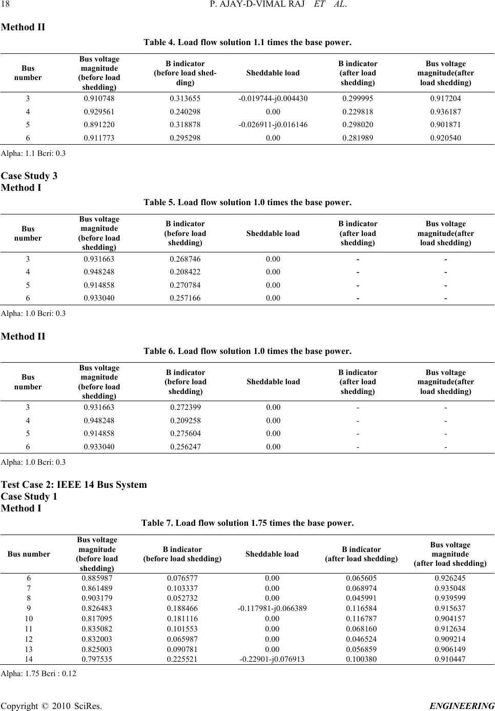

18 P. AJAY-D-VIMAL RAJ ET AL.
Method II
Table 4. Load flow solution 1.1 times the base power.
Bus
number
Bus voltage
magnitude
(before load
shedding)
B indicator
(before load shed-
ding)
Sheddable load
B indicator
(after load
shedding)
Bus voltage
magnitude(after
load shedding)
3 0.910748 0.313655 -0.019744-j0.004430 0.299995 0.917204
4 0.929561 0.240298 0.00 0.229818 0.936187
5 0.891220 0.318878 -0.026911-j0.016146 0.298020 0.901871
6 0.911773 0.295298 0.00 0.281989 0.920540
Alpha: 1.1 Bcri: 0.3
Case Study 3
Method I
Table 5. Load flow solution 1.0 times the base power.
Bus
number
Bus voltage
magnitude
(before load
shedding)
B indicator
(before load
shedding)
Sheddable load
B indicator
(after load
shedding)
Bus voltage
magnitude(after
load shedding)
3 0.931663 0.268746 0.00 - -
4 0.948248 0.208422 0.00 - -
5 0.914858 0.270784 0.00 - -
6 0.933040 0.257166 0.00 - -
Alpha: 1.0 Bcri: 0.3
Method II
Table 6. Load flow solution 1.0 times the base power.
Bus
number
Bus voltage
magnitude
(before load
shedding)
B indicator
(before load
shedding)
Sheddable load
B indicator
(after load
shedding)
Bus voltage
magnitude(after
load shedding)
3 0.931663 0.272399 0.00 - -
4 0.948248 0.209258 0.00 - -
5 0.914858 0.275604 0.00 - -
6 0.933040 0.256247 0.00 - -
Alpha: 1.0 Bcri: 0.3
Test Case 2: IEEE 14 Bus System
Case Study 1
Method I
Table 7. Load flow solution 1.75 times the base power.
Bus number
Bus voltage
magnitude
(before load
shedding)
B indicator
(before load shedding)Sheddable load B indicator (after load shedding)
Bus voltage
magnitude
(after load shedding)
6 0.885987 0.076577 0.00 0.065605 0.926245
7 0.861489 0.103337 0.00 0.068974 0.935048
8 0.903179 0.052732 0.00 0.045991 0.939599
9 0.826483 0.188466 -0.117981-j0.066389 0.116584 0.915637
10 0.817095 0.181116 0.00 0.116787 0.904157
11 0.835082 0.101553 0.00 0.068160 0.912634
12 0.832003 0.065987 0.00 0.046524 0.909214
13 0.825003 0.090781 0.00 0.056859 0.906149
14 0.797535 0.225521 -0.22901-j0.076913 0.100380 0.910447
Alpha: 1.75 Bcri : 0.12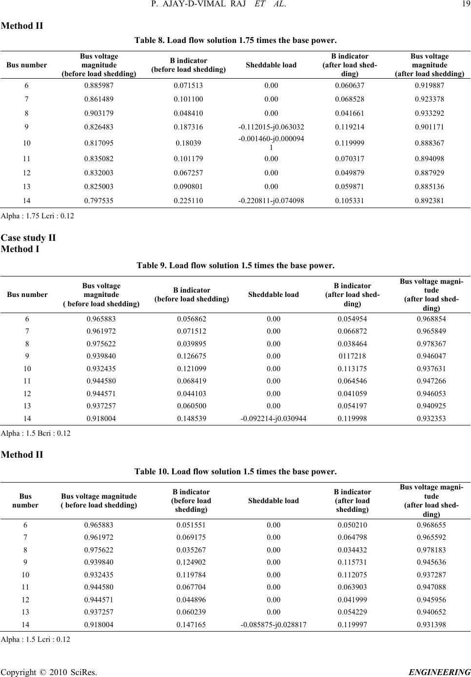

P. AJAY-D-VIMAL RAJ ET AL. 19
Method II
Table 8. Load flow solution 1.75 times the base power.
Bus number
Bus voltage
magnitude
(before load shedding)
B indicator
(before load shedding)Sheddable load
B indicator
(after load shed-
ding)
Bus voltage
magnitude
(after load shedding)
6 0.885987 0.071513 0.00 0.060637 0.919887
7 0.861489 0.101100 0.00 0.068528 0.923378
8 0.903179 0.048410 0.00 0.041661 0.933292
9 0.826483 0.187316 -0.112015-j0.0630320.119214 0.901171
10 0.817095 0.18039
-0.001460-j0.000094
1 0.119999 0.888367
11 0.835082 0.101179 0.00 0.070317 0.894098
12 0.832003 0.067257 0.00 0.049879 0.887929
13 0.825003 0.090801 0.00 0.059871 0.885136
14 0.797535 0.225110 -0.220811-j0.0740980.105331 0.892381
Alpha : 1.75 Lcri : 0.12
Case study II
Method I
Table 9. Load flow solution 1.5 times the base power.
Bus number
Bus voltage
magnitude
( before load shedding)
B indicator
(before load shedding)Sheddable load
B indicator
(after load shed-
ding)
Bus voltage magni-
tude
(after load shed-
ding)
6 0.965883 0.056862 0.00 0.054954 0.968854
7 0.961972 0.071512 0.00 0.066872 0.965849
8 0.975622 0.039895 0.00 0.038464 0.978367
9 0.939840 0.126675 0.00 0117218 0.946047
10 0.932435 0.121099 0.00 0.113175 0.937631
11 0.944580 0.068419 0.00 0.064546 0.947266
12 0.944571 0.044103 0.00 0.041059 0.946053
13 0.937257 0.060500 0.00 0.054197 0.940925
14 0.918004 0.148539 -0.092214-j0.0309440.119998 0.932353
Alpha : 1.5 Bcri : 0.12
Method II
Table 10. Load flow solution 1.5 times the base power.
Bus
number
Bus voltage magnitude
( before load shedding)
B indicator
(before load
shedding)
Sheddable load
B indicator
(after load
shedding)
Bus voltage magni-
tude
(after load shed-
ding)
6 0.965883 0.051551 0.00 0.050210 0.968655
7 0.961972 0.069175 0.00 0.064798 0.965592
8 0.975622 0.035267 0.00 0.034432 0.978183
9 0.939840 0.124902 0.00 0.115731 0.945636
10 0.932435 0.119784 0.00 0.112075 0.937287
11 0.944580 0.067704 0.00 0.063903 0.947088
12 0.944571 0.044896 0.00 0.041999 0.945956
13 0.937257 0.060239 0.00 0.054229 0.940652
14 0.918004 0.147165 -0.085875-j0.0288170.119997 0.931398
Alpha : 1.5 Lcri : 0.12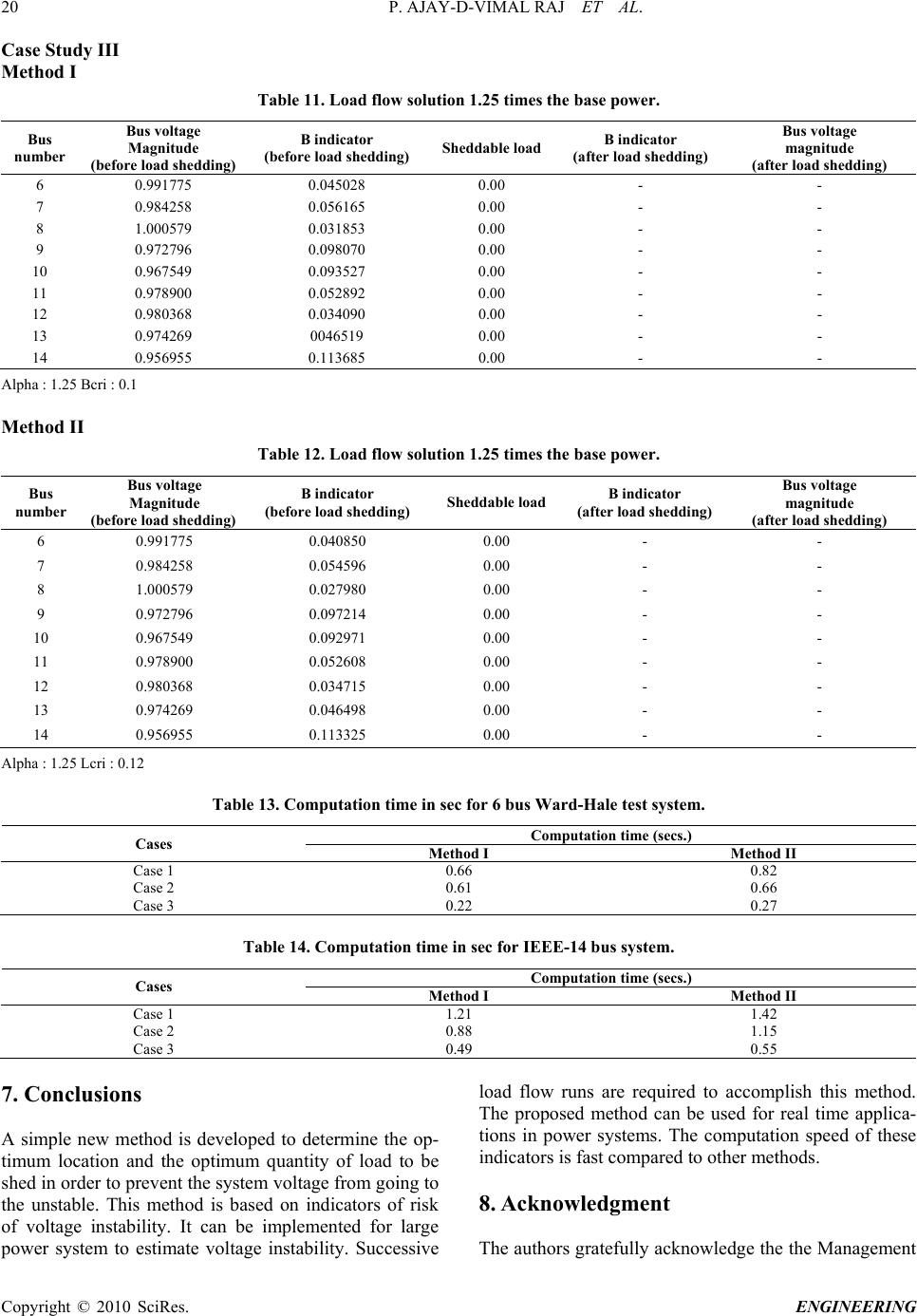

20 P. AJAY-D-VIMAL RAJ ET AL.
Case Study III
Method I
Table 11. Load flow solution 1.25 times the base power.
Bus
number
Bus voltage
Magnitude
(before load shedding)
B indicator
(before load shedding) Sheddable load B indicator (after load shedding)
Bus voltage
magnitude
(after load shedding)
6 0.991775 0.045028 0.00 - -
7 0.984258 0.056165 0.00 - -
8 1.000579 0.031853 0.00 - -
9 0.972796 0.098070 0.00 - -
10 0.967549 0.093527 0.00 - -
11 0.978900 0.052892 0.00 - -
12 0.980368 0.034090 0.00 - -
13 0.974269 0046519 0.00 - -
14 0.956955 0.113685 0.00 - -
Alpha : 1.25 Bcri : 0.1
Method II
Table 12. Load flow solution 1.25 times the base power.
Bus
number
Bus voltage
Magnitude
(before load shedding)
B indicator
(before load shedding) Sheddable load B indicator (after load shedding)
Bus voltage
magnitude
(after load shedding)
6 0.991775 0.040850 0.00 - -
7 0.984258 0.054596 0.00 - -
8 1.000579 0.027980 0.00 - -
9 0.972796 0.097214 0.00 - -
10 0.967549 0.092971 0.00 - -
11 0.978900 0.052608 0.00 - -
12 0.980368 0.034715 0.00 - -
13 0.974269 0.046498 0.00 - -
14 0.956955 0.113325 0.00 - -
Alpha : 1.25 Lcri : 0.12
Table 13. Computation time in sec for 6 bus Ward-Hale test system.
Computation time (secs.)
Cases Method I Method II
Case 1 0.66 0.82
Case 2 0.61 0.66
Case 3 0.22 0.27
Table 14. Computation time in sec for IEEE-14 bus system.
Computation time (secs.)
Cases Method I Method II
Case 1 1.21 1.42
Case 2 0.88 1.15
Case 3 0.49 0.55
7. Conclusions
A simple new method is developed to determine the op-
timum location and the optimum quantity of load to be
shed in order to prevent the system voltage from going to
the unstable. This method is based on indicators of risk
of voltage instability. It can be implemented for large
power system to estimate voltage instability. Successive
load flow runs are required to accomplish this method.
The proposed method can be used for real time applica-
tions in power systems. The computation speed of these
indicators is fast compared to other methods.
8. Acknowledgment
The authors gratefully acknowledge the the Management

P. AJAY-D-VIMAL RAJ ET AL. 21
of Pondicherry Engineering College, Pondicherry, IN-
DIA for their continued support, encouragement and the
facilities provided to carry out this research work.
9
. References
[1] C. W. Taylor, “Concept of under voltage load shedding
for voltage stability,” IEEE transactions on Power Deliv-
ery, Vol. 7, No. 2, pp. 480–488, 1992
[2] S. A. Niern berg, D. A. Meinnis, and K. D. Sparks, “Fast
acting load shedding,” IEEE Transactions on Power Sys-
tems, Vol. 7, No. 2, pp. 873–877, 1992.
[3] P. Kessel and H. Glavitsch, “Estimating the voltage sta-
bility of a power system,” IEEE Transactions on Power
Delivery, Vol. 1, No. 3, pp. 346–354, 1986,
[4] T. Quoc Taun, J. Fandino, N. Hadjsaid, and J. C. sabon-
nadiere, H. Vu, “Emergency load shedding to avoid risks
of voltage instability using indicators,” IEEE Transac-
tions on Power Systems, Vol. 9, No. 1, pp. 341–351,
1994.
[5] T. Quoc Taun, J. Fandino, N. Hadjsaid, and J. C. sabon-
nadiere, “Fast calculation of indicators of risk of voltage
instability,” Proc .of 27th Universities Power Engineering
Conference, UPEC–92 , pp. 612–615, 1992.
[6] C. W. Taylor, “Power system voltage stability,” Mc.Graw
Hill, 1993.
[7] L. P. Hajdu, J. Peschon, W. F. Tinney, and D. S. Piercy,
“Optimum load-shedding policy for power system,” IEEE
Tran, PAS-87, No. 3, pp. 784–794, 1968.
[8] D. K. Subramanian, “Optimum load shedding through
programming techniques,” IEEE Trans, PAS-90, pp.
89–94, 1971.
[9] S. M. Chan and F. C. Schweppe, “A generation relloca-
tion and load shedding algorithm,” IEEE Trans., PAS-98,
No. 1, pp. 26–34, 1979.
[10] M. M. Adibi and D. K. Thorne, “Local load shedding,”
IEEE Trans. On Power System, Vol. 3, No. 3, pp.
1220–1226, 1988.
[11] S. Shah and S. M. Shahldehpour, “A heuristic approach
to load shedding scheme,” IEEE Trans, on Power System,
Vol. 4, No. 4, pp. 1421–1429, 1989.
[12] R. Billinton and J. Satish, “Effect of rotational load shed-
ding on overall power system adequacy indices,” IEE
Proc. C, Vol. 143, No. 2, pp. 181–187, 1996.
[13] P. Wang and R. Billinton, “Optimum load-shedding tech-
nique to reduce the total customer interruption cost in a
distribution system,” IEE Proc. - Gener. Transm. Distrib.,
Vol. 147, No. 1, pp. 51–56, 2000.
[14] D. Xu and A. A. Girgis, “Optimal Load Shedding Strat-
egy in Power Systems with Distributed Generation,”
IEEE, pp. 788–793, 2001.
[15] Y. Lu, W. S. Kao, and Y. T. Chen, “Study of applying
load shedding scheme with dynamic d-factor values of
various dynamic load models to taiwan power system,”
IEEE Transactions on Power Systems, Vol. 20, No. 4, pp.
1976–1984, 2005.
[16] R. Faranda, A. Pievatolo, and E. Tironi, “Load shedding:
A new proposal,” IEEE Transactions on Power Systems,
Vol. 22, No. 4, pp. 2086–2093, 2007.
[17] A. Wiszniewski, “New criteria of voltage stability margin
for the purpose of load shedding,” IEEE Transactions on
Power Delivery, Vol. 22, No. 3, pp. 1367–1371, 2007.
[18] Z. P. Ding, S. K. Srivastava, D. A. Cartes, and S. Sury-
anarayanan, “Dynamic simulation-based analysis of a
new load shedding scheme for a notional destroyer-class
shipboard power system,” IEEE Transactions on Industry
Applications, Vol. 45, No. 3, pp. 1163–1174, 2009.
[19] E. J. Thalassinakis, E. N. Dialynas, and D. Agoris,
“Method combining anns and monte carlo simulation for
the selection of the load shedding protection strategies in
autonomous power systems,” IEEE Transactions on
Power Systems, Vol. 21, No. 4, pp. 1574–1582. 2006.