Paper Menu >>
Journal Menu >>
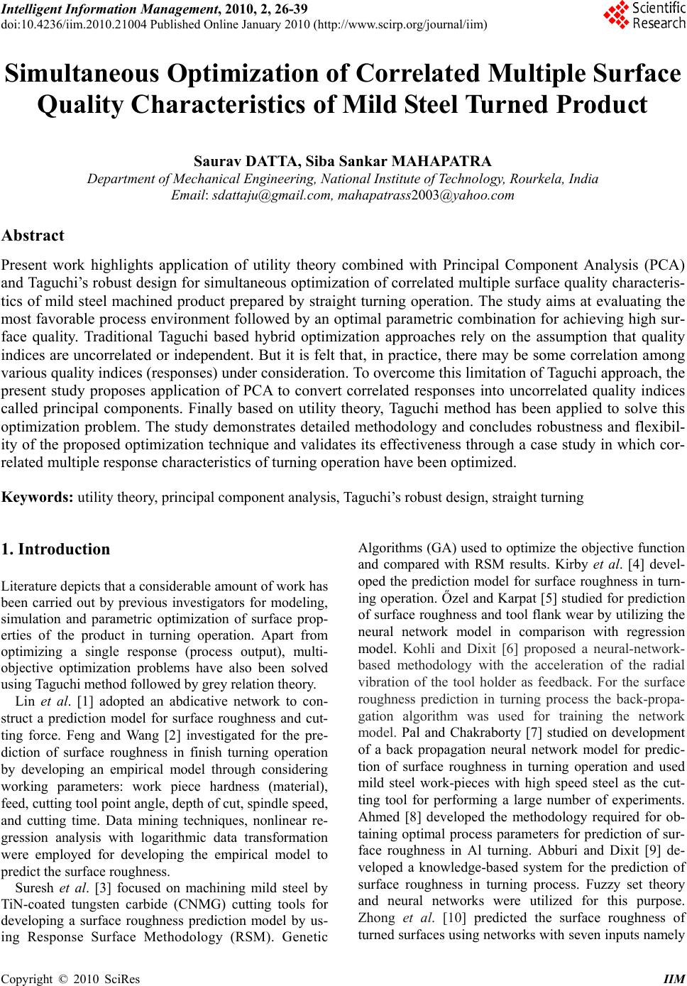 Intelligent Information Management, 2010, 2, 26-39 doi:10.4236/iim.2010.21004 Published Online January 2010 (http://www.scirp.org/journal/iim) Copyright © 2010 SciRes IIM Simultaneous Optimization of Correlated Multiple Surface Quality Characteristics of Mild Steel Turned Product Saurav DATTA, Siba Sankar MAHAPATRA Department of Mechanical Engineering, National Institute of Technology, Rourkela, India Email: sdattaju@gmail.com, mahapatrass20 03@yahoo.com Abstract Present work highlights application of utility theory combined with Principal Component Analysis (PCA) and Taguchi’s robust design for simultaneous optimization of correlated multiple surface quality characteris- tics of mild steel machined product prepared by straight turning operation. The study aims at evaluating the most favorable process environment followed by an optimal parametric combination for achieving high sur- face quality. Traditional Taguchi based hybrid optimization approaches rely on the assumption that quality indices are uncorrelated or independent. But it is felt that, in practice, there may be some correlation among various quality indices (responses) under consideration. To overcome this limitation of Taguchi approach, the present study proposes application of PCA to convert correlated responses into uncorrelated quality indices called principal components. Finally based on utility theory, Taguchi method has been applied to solve this optimization problem. The study demonstrates detailed methodology and concludes robustness and flexibil- ity of the proposed optimization technique and validates its effectiveness through a case study in which cor- related multiple response characteristics of turning operation have been optimized. Keywords: utility theory, principal component analysis, Taguchi’s robust design, straight turning 1. Introduction Literature depicts that a considerable amount of work has been carried out by previous investigators for modeling, simulation and parametric optimization of surface prop- erties of the product in turning operation. Apart from optimizing a single response (process output), multi- objective optimization problems have also been solved using Taguchi method followed by grey relation theory. Lin et al. [1] adopted an abdicative network to con- struct a prediction model for surface roughness and cut- ting force. Feng and Wang [2] investigated for the pre- diction of surface roughness in finish turning operation by developing an empirical model through considering working parameters: work piece hardness (material), feed, cutting tool point angle, depth of cut, spindle speed, and cutting time. Data mining techniques, nonlinear re- gression analysis with logarithmic data transformation were employed for developing the empirical model to predict the surface roughness. Suresh et al. [3] focused on machining mild steel by TiN-coated tungsten carbide (CNMG) cutting tools for developing a surface roughness prediction model by us- ing Response Surface Methodology (RSM). Genetic Algorithms (GA) used to optimize the objective function and compared with RSM results. Kirby et al. [4] devel- oped the prediction model for surface roughness in turn- ing operation. Őzel and Karpat [5] studied for prediction of surface roughness and tool flank wear by utilizing the neural network model in comparison with regression model. Kohli and Dixit [6] proposed a neural-network- based methodology with the acceleration of the radial vibration of the tool holder as feedback. For the surface roughness prediction in turning process the back-propa- gation algorithm was used for training the network model. Pal and Chakraborty [7] studied on development of a back propagation neural network model for predic- tion of surface roughness in turning operation and used mild steel work-pieces with high speed steel as the cut- ting tool for performing a large number of experiments. Ahmed [8] developed the methodology required for ob- taining optimal process parameters for prediction of sur- face roughness in Al turning. Abburi and Dixit [9] de- veloped a knowledge-based system for the prediction of surface roughness in turning process. Fuzzy set theory and neural networks were utilized for this purpose. Zhong et al. [10] predicted the surface roughness of turned surfaces using networks with seven inputs namely 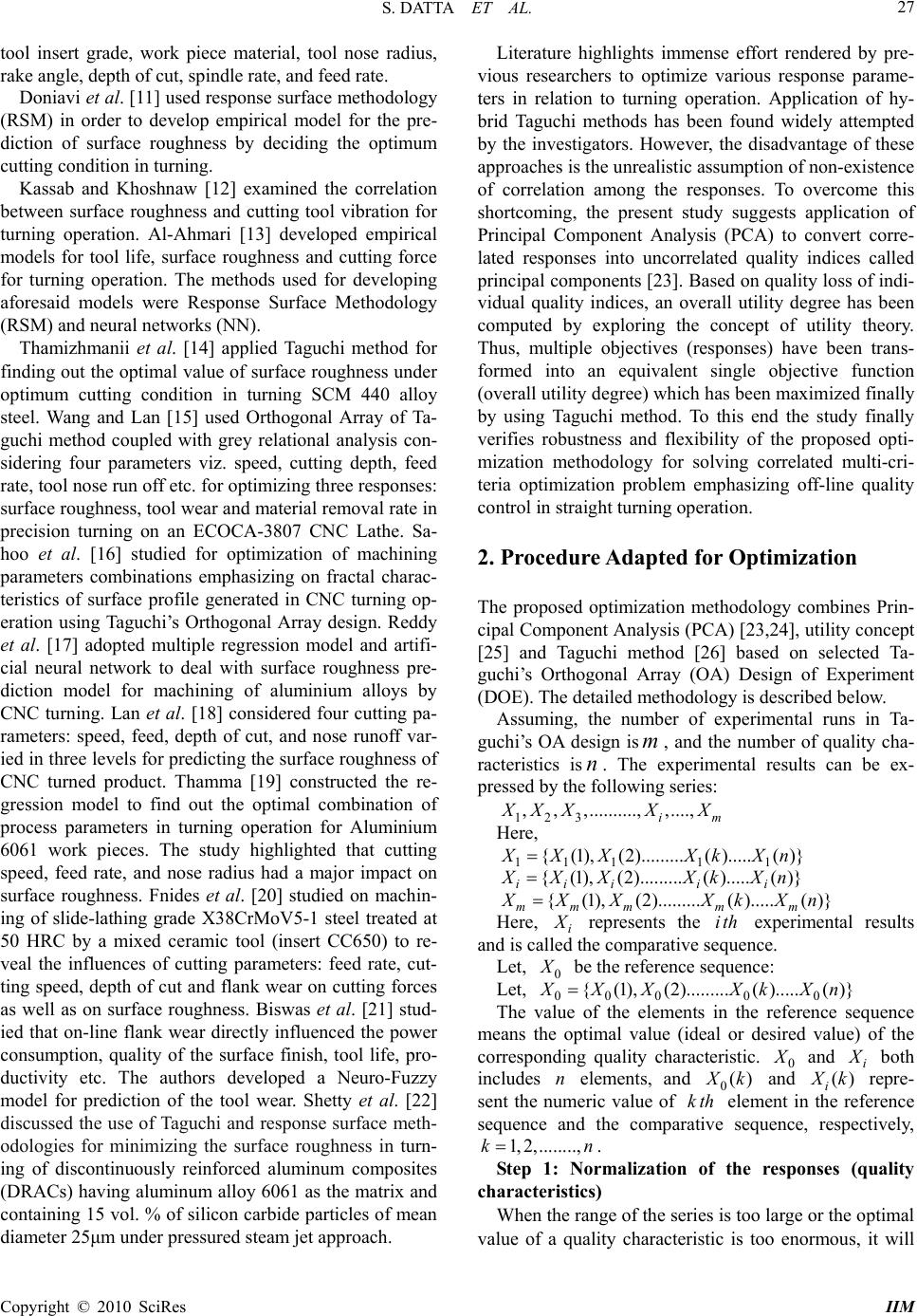 S. DATTA ET AL. 27 tool insert grade, work piece material, tool nose radius, rake angle, depth of cut, spindle rate, and feed rate. Doniavi et al. [11] used response surface methodology (RSM) in order to develop empirical model for the pre- diction of surface roughness by deciding the optimum cutting condition in turning. Kassab and Khoshnaw [12] examined the correlation between surface roughness and cutting tool vibration for turning operation. Al-Ahmari [13] developed empirical models for tool life, surface roughness and cutting force for turning operation. The methods used for developing aforesaid models were Response Surface Methodology (RSM) and neural networks (NN). Thamizhmanii et al. [14] applied Taguchi method for finding out the optimal value of surface roughness under optimum cutting condition in turning SCM 440 alloy steel. Wang and Lan [15] used Orthogonal Array of Ta- guchi method coupled with grey relational analysis con- sidering four parameters viz. speed, cutting depth, feed rate, tool nose run off etc. for optimizing three responses: surface roughness, tool wear and material removal rate in precision turning on an ECOCA-3807 CNC Lathe. Sa- hoo et al. [16] studied for optimization of machining parameters combinations emphasizing on fractal charac- teristics of surface profile generated in CNC turning op- eration using Taguchi’s Orthogonal Array design. Reddy et al. [17] adopted multiple regression model and artifi- cial neural network to deal with surface roughness pre- diction model for machining of aluminium alloys by CNC turning. Lan et al. [18] considered four cutting pa- rameters: speed, feed, depth of cut, and nose runoff var- ied in three levels for predicting the surface roughness of CNC turned product. Thamma [19] constructed the re- gression model to find out the optimal combination of process parameters in turning operation for Aluminium 6061 work pieces. The study highlighted that cutting speed, feed rate, and nose radius had a major impact on surface roughness. Fnides et al. [20] studied on machin- ing of slide-lathing grade X38CrMoV5-1 steel treated at 50 HRC by a mixed ceramic tool (insert CC650) to re- veal the influences of cutting parameters: feed rate, cut- ting speed, depth of cut and flank wear on cutting forces as well as on surface roughness. Biswas et al. [21] stud- ied that on-line flank wear directly influenced the power consumption, quality of the surface finish, tool life, pro- ductivity etc. The authors developed a Neuro-Fuzzy model for prediction of the tool wear. Shetty et al. [22] discussed the use of Taguchi and response surface meth- odologies for minimizing the surface roughness in turn- ing of discontinuously reinforced aluminum composites (DRACs) having aluminum alloy 6061 as the matrix and containing 15 vol. % of silicon carbide particles of mean diameter 25μm under pressured steam jet approach. Literature highlights immense effort rendered by pre- vious researchers to optimize various response parame- ters in relation to turning operation. Application of hy- brid Taguchi methods has been found widely attempted by the investigators. However, the disadvantage of these approaches is the unrealistic assumption of non-existence of correlation among the responses. To overcome this shortcoming, the present study suggests application of Principal Component Analysis (PCA) to convert corre- lated responses into uncorrelated quality indices called principal components [23]. Based on quality loss of indi- vidual quality indices, an overall utility degree has been computed by exploring the concept of utility theory. Thus, multiple objectives (responses) have been trans- formed into an equivalent single objective function (overall utility degree) which has been maximized finally by using Taguchi method. To this end the study finally verifies robustness and flexibility of the proposed opti- mization methodology for solving correlated multi-cri- teria optimization problem emphasizing off-line quality control in straight turning operation. 2. Procedure Adapted for Optimization The proposed optimization methodology combines Prin- cipal Component Analysis (PCA) [23,24], utility concept [25] and Taguchi method [26] based on selected Ta- guchi’s Orthogonal Array (OA) Design of Experiment (DOE). The detailed methodology is described below. Assuming, the number of experimental runs in Ta- guchi’s OA design is, and the number of quality cha- racteristics is. The experimental results can be ex- pressed by the following series: m n 123 ,,,.........., ,...., im X XXX X Here, 1111 1 {(1),(2).........( ).....( )} X XXXk Xn { (1),(2)......... ()..... ()} iiii i X XXXk Xn { (1),(2)......... ()..... ()} mmmm m X XXXk Xn Here, i X represents the experimental results and is called the comparative sequence. ith Let, 0 X be the reference sequence: Let, 0000 0 { (1),(2)......... ()..... ()} X XX XkXn The value of the elements in the reference sequence means the optimal value (ideal or desired value) of the corresponding quality characteristic. 0 X and i X both includes elements, and 0 n() X k and i() X k repre- sent the numeric value of element in the reference sequence and the comparative sequence, respectively, kth 1,2,.. ,kn...... . Step 1: Normalization of the responses (quality characteristics) When the range of the series is too large or the optimal value of a quality characteristic is too enormous, it will Copyright © 2010 SciRes IIM 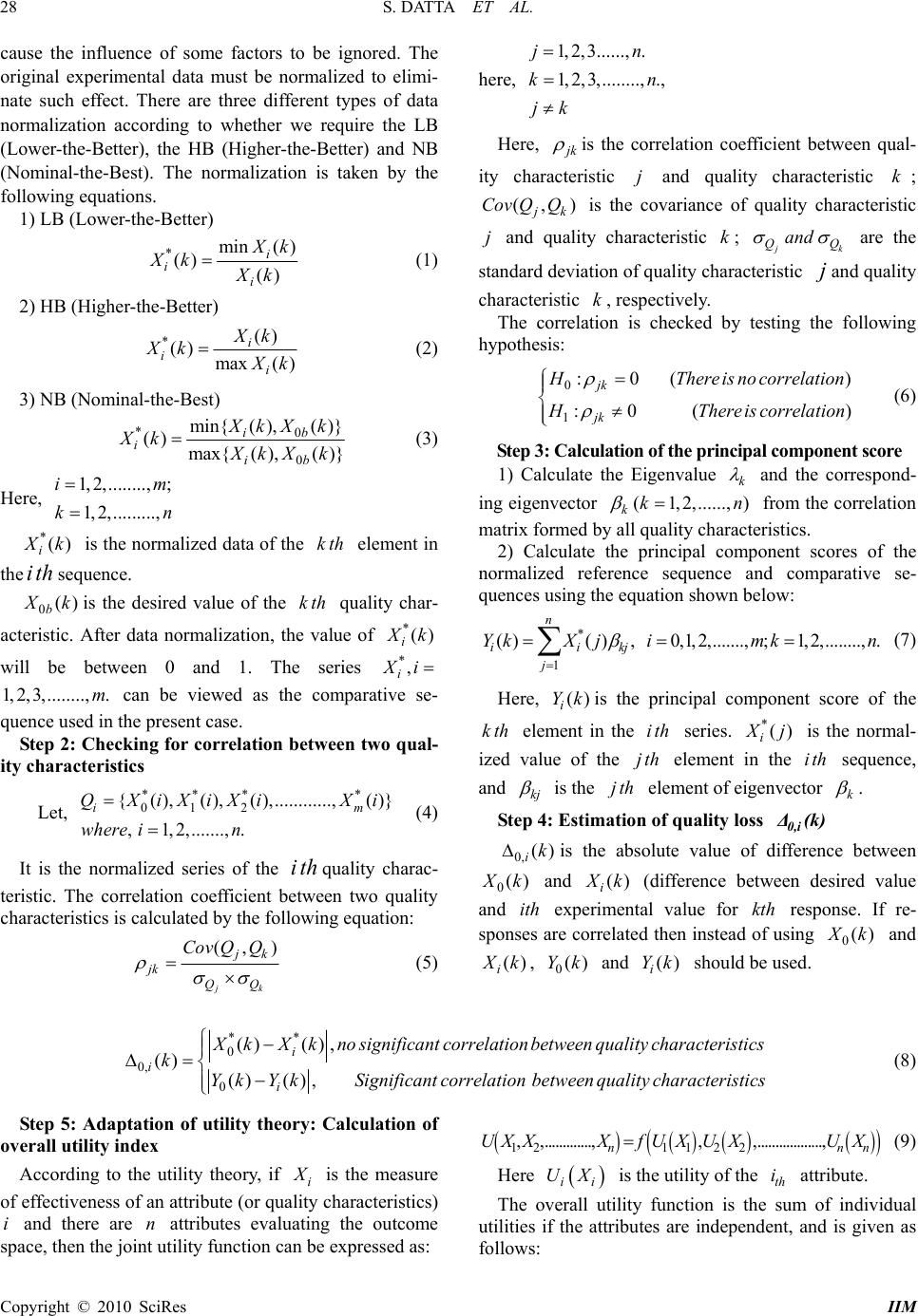 S. DATTA ET AL. Copyright © 2010 SciRes IIM 28 here, 1,2,3......, . 1,2,3,........, ., jn kn jk cause the influence of some factors to be ignored. The original experimental data must be normalized to elimi- nate such effect. There are three different types of data normalization according to whether we require the LB (Lower-the-Better), the HB (Higher-the-Better) and NB (Nominal-the-Best). The normalization is taken by the following equations. Here, j k is the correlation coefficient between qual- ity characteristic and quality characteristic k; is the covariance of quality characteristic and quality characteristic ; j (,Cov Q j ) jk Q k j k Q and 1) LB (Lower-the-Better) Q are the standard deviation of quality characteristic j and quality characteristic , respectively. k *min( ) () () i i i X k Xk Xk (1) 2) HB (Higher-the-Better) The correlation is checked by testing the following hypothesis: *() () max( ) i i i X k Xk X k (2) 0 1 :0( :0 ( jk jk ) ) H Thereis no correlation H Thereis correlation (6) 3) NB (Nominal-the-Best) *0 0 min{( ),( )} () max{( ),( )} ib i ib X kX k Xk X kX k (3) Step 3: Calculation of the principal component score 1) Calculate the Eigenvalue k and the correspond- ing eigenvector ( 1,2,.... kk.., ) Here, 1,2,........, ; 1,2,........., im kn n from the correlation matrix formed by all quality characteristics. *() i X k ith is the normalized data of the element in the sequence. kth 2) Calculate the principal component scores of the normalized reference sequence and comparative se- quences using the equation shown below: 0() b X kis the desired value of the quality char- acteristic. After data normalization, the value of kth *() i X k *, i will be between 0 and 1. The series X i can be viewed as the comparative se- quence used in the present case. 1, .m2,3,........, * 1 ( )( ),0,1,2,.......,;1,2,........,. n iikj j YkX jimkn (7) Step 2: Checking for correlation between two qual- ity characteristics Let, (4) *** * 01 2 {(),( ),( ),............,( )} ,1,2,.......,. i QX iXiXiXi wherein m Here, is the principal component score of the element in the series. () i Yk kth ith*() i X j is the normal- ized value of the element in the sequence, and jth ith kj is the element of eigenvector jth k . Step 4: Estimation of quality loss 0,i Δ(k) 0, () ik is the absolute value of difference between 0() X k and () i X k (difference between desired value and experimental value for response. If re- sponses are correlated then instead of using ithkth 0() X k and () i X k0 Y, and should be used. ()k() i Yk It is the normalized series of the quality charac- teristic. The correlation coefficient between two quality characteristics is calculated by the following equation: ith (,) jk jk jk QQ CovQQ (5) ** 0 0, 0 ()(), () () (), i i i X kX knosignificantcorrelationbetweenqualitycharacteristics k YkYkSignificantcorrelationbetween quality characteristics (8) Step 5: Adaptation of utility theory: Calculation of overall utility index 12112 2 , ,.............,,,.................., nn UX XXfUXUXUXn (9) Here ii UX is the utility of the attribute. th i According to the utility theory, if i X is the measure of effectiveness of an attribute (or quality characteristics) and there are attributes evaluating the outcome space, then the joint utility function can be expressed as: in The overall utility function is the sum of individual utilities if the attributes are independent, and is given as follows: 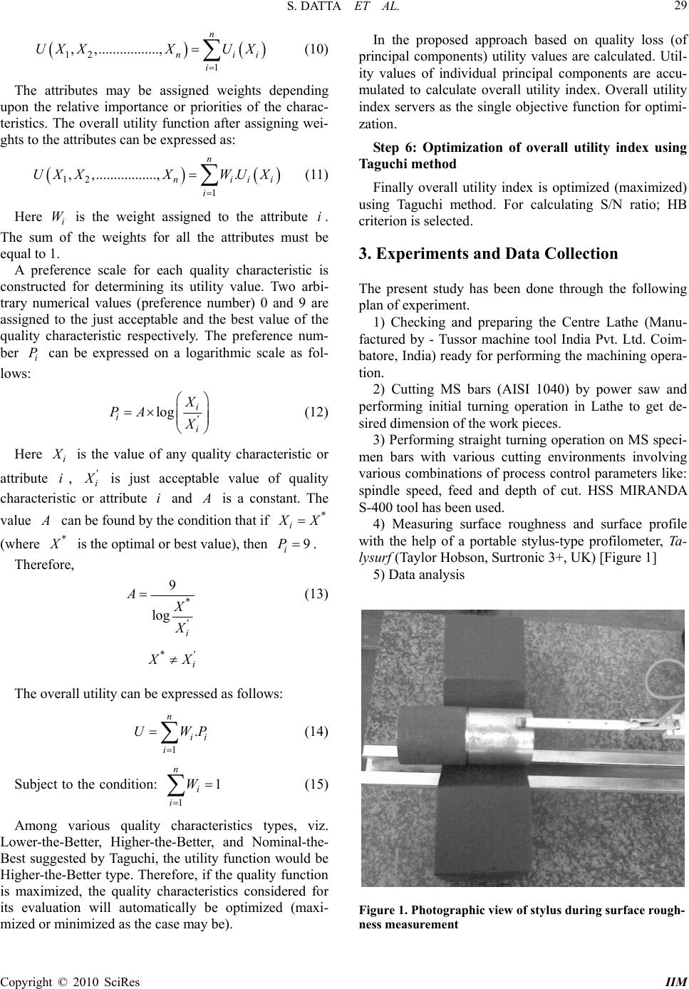 S. DATTA ET AL. 29 12 1 , ,................., n ni i UX XXUX i i (10) The attributes may be assigned weights depending upon the relative importance or priorities of the charac- teristics. The overall utility function after assigning wei- ghts to the attributes can be expressed as: 12 1 , ,.................,. n nii i UX XXWUX (11) Here is the weight assigned to the attribute . The sum of the weights for all the attributes must be equal to 1. i W i A preference scale for each quality characteristic is constructed for determining its utility value. Two arbi- trary numerical values (preference number) 0 and 9 are assigned to the just acceptable and the best value of the quality characteristic respectively. The preference num- ber can be expressed on a logarithmic scale as fol- lows: i P ' log i i i X PA X (12) Here i X is the value of any quality characteristic or attribute , i' i X is just acceptable value of quality characteristic or attribute and i A is a constant. The value A can be found by the condition that if * i X X (where * X is the optimal or best value), then 9 i P . Therefore, * ' 9 log i A X X (13) *' i X X The overall utility can be expressed as follows: 1 . n ii i UW P (14) Subject to the condition: (15) 1 1 n i i W Among various quality characteristics types, viz. Lower-the-Better, Higher-the-Better, and Nominal-the- Best suggested by Taguchi, the utility function would be Higher-the-Better type. Therefore, if the quality function is maximized, the quality characteristics considered for its evaluation will automatically be optimized (maxi- mized or minimized as the case may be). In the proposed approach based on quality loss (of principal components) utility values are calculated. Util- ity values of individual principal components are accu- mulated to calculate overall utility index. Overall utility index servers as the single objective function for optimi- zation. Step 6: Optimization of overall utility index using Taguchi method Finally overall utility index is optimized (maximized) using Taguchi method. For calculating S/N ratio; HB criterion is selected. 3. Experiments and Data Collection The present study has been done through the following plan of experiment. 1) Checking and preparing the Centre Lathe (Manu- factured by - Tussor machine tool India Pvt. Ltd. Coim- batore, India) ready for performing the machining opera- tion. 2) Cutting MS bars (AISI 1040) by power saw and performing initial turning operation in Lathe to get de- sired dimension of the work pieces. 3) Performing straight turning operation on MS speci- men bars with various cutting environments involving various combinations of process control parameters like: spindle speed, feed and depth of cut. HSS MIRANDA S-400 tool has been used. 4) Measuring surface roughness and surface profile with the help of a portable stylus-type profilometer, Ta- lysurf (Taylor Hobson, Surtronic 3+, UK) [Figure 1] 5) Data analysis Figure 1. Photographic view of stylus during surface rough- ness measurement Copyright © 2010 SciRes IIM 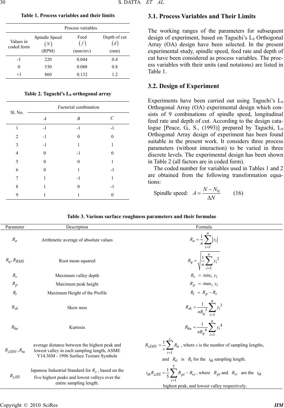 S. DATTA ET AL. Copyright © 2010 SciRes IIM 30 3.1. Process Variables and Their Limits Table 1. Process variables and their limits Process variables Values in coded form Spindle Speed N (RPM) Feed f (mm/rev) Depth of cut d (mm) -1 220 0.044 0.4 0 530 0.088 0.8 +1 860 0.132 1.2 The working ranges of the parameters for subsequent design of experiment, based on Taguchi’s L9 Orthogonal Array (OA) design have been selected. In the present experimental study, spindle speed, feed rate and depth of cut have been considered as process variables. The proc- ess variables with their units (and notations) are listed in Table 1. 3.2. Design of Experiment Table 2. Taguchi’s L9 orthogonal array Experiments have been carried out using Taguchi’s L9 Orthogonal Array (OA) experimental design which con- sists of 9 combinations of spindle speed, longitudinal feed rate and depth of cut. According to the design cata- logue [Peace, G., S., (1993)] prepared by Taguchi, L9 Orthogonal Array design of experiment has been found suitable in the present work. It considers three process parameters (without interaction) to be varied in three discrete levels. The experimental design has been shown in Table 2 (all factors are in coded form). Factorial combination Sl. No. A B C 1 -1 -1 -1 2 -1 0 0 3 -1 1 1 4 0 -1 0 5 0 0 1 6 0 1 -1 7 1 -1 1 8 1 0 -1 9 1 1 0 The coded number for variables used in Tables 1 and 2 are obtained from the following transformation equa- tions: Spindle speed: 0 NN AN (16) Table 3. Various surface roughness parameters and their formulae Parameter Description Formula a R Arithmetic average of absolute values 1 1n ai i R y n , qRMS RR Root mean squared 2 1 1n qi i R y n v R Maximum valley depth min vii R y p R Maximum peak height max pii R y t R Maximum Height of the Profile tpv R RR s k R Skew ness 3 3 1 1n s ki qi R y nR ku R Kurtosis 4 4 1 1n ku i qi R y nR , zDIN m R R average distance between the highest peak and lowest valley in each sampling length, ASME Y14.36M - 1996 Surface Texture Symbols 1 1 s zDIN ti i R R s , where s is the number of sampling lengths, and ti R is t R for the sampling length. th i zJIS R Japanese Industrial Standard forz R , based on the five highest peaks and lowest valleys over the entire sampling length. 5 1 1 5 th zJISpivi i iRR R , where pi R and vi R are the th i highest peak, and lowest valley respectively. 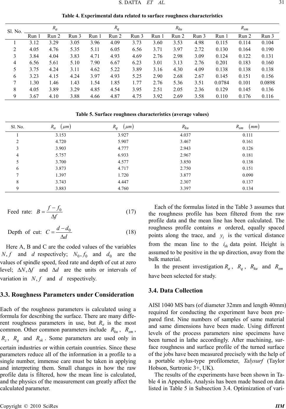 S. DATTA ET AL. 31 Table 4. Experimental data related to surface roughness characteristics a R q R ku R s m R Sl. No. Run 1 Run 2 Run 3 Run 1 Run 2Run 3Run 1Run 2Run 3Run 1 Run 2 Run 3 1 3.12 3.29 3.05 3.96 4.09 3.73 3.603.53 4.98 0.115 0.114 0.104 2 4.05 4.76 5.35 5.11 6.05 6.56 3.713.97 2.72 0.130 0.164 0.190 3 3.84 4.04 3.83 4.71 4.93 4.69 2.762.98 3.09 0.124 0.122 0.131 4 6.56 5.61 5.10 7.90 6.67 6.23 3.013.13 2.76 0.201 0.183 0.160 5 3.75 4.24 3.11 4.62 5.22 3.89 3.164.30 4.09 0.138 0.138 0.138 6 3.23 4.15 4.24 3.97 4.93 5.25 2.902.68 2.67 0.145 0.151 0.156 7 1.30 1.46 1.43 1.54 1.85 1.77 2.765.36 3.51 0.0784 0.101 0.0898 8 4.05 3.89 3.29 4.85 4.54 3.95 2.512.05 2.36 0.129 0.145 0.136 9 3.67 4.10 3.88 4.66 4.87 4.75 3.922.69 3.58 0.110 0.176 0.116 Table 5. Surface roughness characteristics (average values) Sl. No. a R m q R m ku R s m R mm 1 3.153 3.927 4.037 0.111 2 4.720 5.907 3.467 0.161 3 3.903 4.777 2.943 0.126 4 5.757 6.933 2.967 0.181 5 3.700 4.577 3.850 0.138 6 3.873 4.717 2.750 0.151 7 1.397 1.720 3.877 0.090 8 3.743 4.447 2.307 0.137 9 3.883 4.760 3.397 0.134 Feed rate: 0 f f B f (17) Depth of cut: 0 dd Cd (18) Here A, B and C are the coded values of the variables and respectively; and are the values of spindle speed, feed rate and depth of cut at zero level; and are the units or intervals of variation in and respectively. ,Nf d Nf ,N 00 ,Nf 0 d ,d df 3.3. Roughness Parameters under Consideration Each of the roughness parameters is calculated using a formula for describing the surface. There are many diffe- rent roughness parameters in use, but Ra is the most common. Other common parameters include , ku R s m R, , and z Rq R s k R. Some parameters are used only in certain industries or within certain countries. Since these parameters reduce all of the information in a profile to a single number, immense care must be taken in applying and interpreting them. Small changes in how the raw profile data is filtered, how the mean line is calculated, and the physics of the measurement can greatly affect the calculated parameter. Each of the formulas listed in the Table 3 assumes that the roughness profile has been filtered from the raw profile data and the mean line has been calculated. The roughness profile contains ordered, equally spaced points along the trace, and is the vertical distance from the mean line to the data point. Height is assumed to be positive in the up direction, away from the bulk material. n i y ith In the present investigation, , and a Rq Rku R s m R have been selected for study. 3.4. Data Collection AISI 1040 MS bars (of diameter 32mm and length 40mm) required for conducting the experiment have been pre- pared first. Nine numbers of samples of same material and same dimensions have been made. Using different levels of the process parameters nine specimens have been turned in lathe accordingly. After machining, sur- face roughness and surface profile of the turned surface of the jobs have been measured precisely with the help of a portable stylus-type profilometer, Talysurf (Taylor Hobson, Surtronic 3+, UK). The results of the experiments have been shown in Ta- ble 4 in Appendix. Analysis has been made based on data listed in Table 5 in Subsection 3.4. Optimization of vari- Copyright © 2010 SciRes IIM 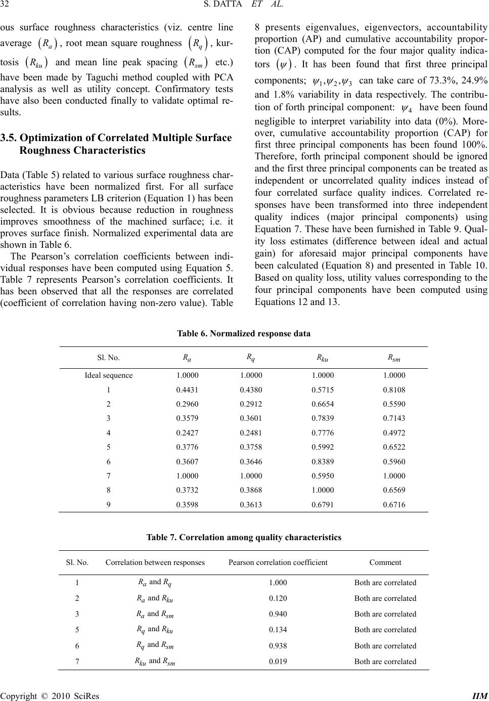 S. DATTA ET AL. 32 ous surface roughness characteristics (viz. centre line average , root mean square roughness a R q R, kur- tosis and mean line peak spacing ku R s m R etc.) have been made by Taguchi method coupled with PCA analysis as well as utility concept. Confirmatory tests have also been conducted finally to validate optimal re- sults. 3.5. Optimization of Correlated Multiple Surface Roughness Characteristics Data (Table 5) related to various surface roughness char- acteristics have been normalized first. For all surface roughness parameters LB criterion (Equation 1) has been selected. It is obvious because reduction in roughness improves smoothness of the machined surface; i.e. it proves surface finish. Normalized experimental data are shown in Table 6. The Pearson’s correlation coefficients between indi- vidual responses have been computed using Equation 5. Table 7 represents Pearson’s correlation coefficients. It has been observed that all the responses are correlated (coefficient of correlation having non-zero value). Table 8 presents eigenvalues, eigenvectors, accountability proportion (AP) and cumulative accountability propor- tion (CAP) computed for the four major quality indica- tors . It has been found that first three principal components; 123 ,, can take care of 73.3%, 24.9% and 1.8% variability in data respectively. The contribu- tion of forth principal component: 4 have been found negligible to interpret variability into data (0%). More- over, cumulative accountability proportion (CAP) for first three principal components has been found 100%. Therefore, forth principal component should be ignored and the first three principal components can be treated as independent or uncorrelated quality indices instead of four correlated surface quality indices. Correlated re- sponses have been transformed into three independent quality indices (major principal components) using Equation 7. These have been furnished in Table 9. Qual- ity loss estimates (difference between ideal and actual gain) for aforesaid major principal components have been calculated (Equation 8) and presented in Table 10. Based on quality loss, utility values corresponding to the four principal components have been computed using Equations 12 and 13. Table 6. Normalized response data Sl. No. a R q R ku R s m R Ideal sequence 1.0000 1.0000 1.0000 1.0000 1 0.4431 0.4380 0.5715 0.8108 2 0.2960 0.2912 0.6654 0.5590 3 0.3579 0.3601 0.7839 0.7143 4 0.2427 0.2481 0.7776 0.4972 5 0.3776 0.3758 0.5992 0.6522 6 0.3607 0.3646 0.8389 0.5960 7 1.0000 1.0000 0.5950 1.0000 8 0.3732 0.3868 1.0000 0.6569 9 0.3598 0.3613 0.6791 0.6716 Table 7. Correlation among quality characteristics Sl. No. Correlation between responses Pearson correlation coefficient Comment 1 a R and q R 1.000 Both are correlated 2 a R and ku R 0.120 Both are correlated 3 a R and s m R 0.940 Both are correlated 5 q R and ku R 0.134 Both are correlated 6 q R and s m R 0.938 Both are correlated 7 ku R and s m R 0.019 Both are correlated Copyright © 2010 SciRes IIM 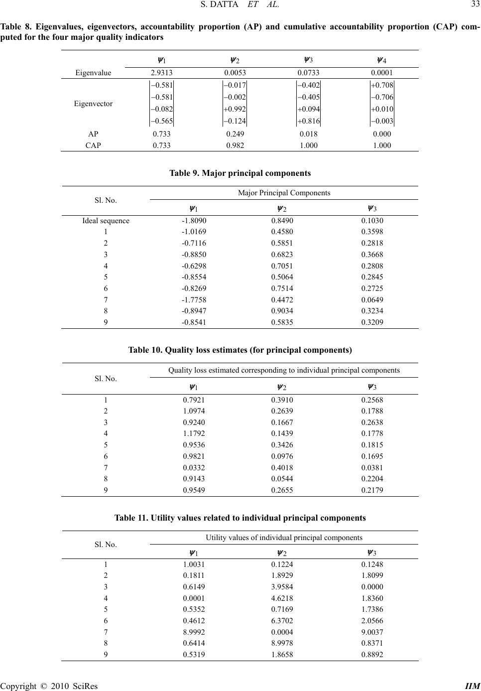 S. DATTA ET AL. 33 Table 8. Eigenvalues, eigenvectors, accountability proportion (AP) and cumulative accountability proportion (CAP) com- puted for the four major quality indicators 1 2 3 4 Eigenvalue 2.9313 0.0053 0.0733 0.0001 Eigenvector 0.581 0.581 0.082 0.565 0.017 0.002 0.992 0.124 0.402 0.405 0.094 0.816 0.708 0.706 0.010 0.003 AP 0.733 0.249 0.018 0.000 CAP 0.733 0.982 1.000 1.000 Table 9. Major principal components Major Principal Components Sl. No. 1 2 3 Ideal sequence -1.8090 0.8490 0.1030 1 -1.0169 0.4580 0.3598 2 -0.7116 0.5851 0.2818 3 -0.8850 0.6823 0.3668 4 -0.6298 0.7051 0.2808 5 -0.8554 0.5064 0.2845 6 -0.8269 0.7514 0.2725 7 -1.7758 0.4472 0.0649 8 -0.8947 0.9034 0.3234 9 -0.8541 0.5835 0.3209 Table 10. Quality loss estimates (for principal components) Quality loss estimated corresponding to individual principal components Sl. No. 1 2 3 1 0.7921 0.3910 0.2568 2 1.0974 0.2639 0.1788 3 0.9240 0.1667 0.2638 4 1.1792 0.1439 0.1778 5 0.9536 0.3426 0.1815 6 0.9821 0.0976 0.1695 7 0.0332 0.4018 0.0381 8 0.9143 0.0544 0.2204 9 0.9549 0.2655 0.2179 Table 11. Utility values related to individual principal components Utility values of individual principal components Sl. No. 1 2 3 1 1.0031 0.1224 0.1248 2 0.1811 1.8929 1.8099 3 0.6149 3.9584 0.0000 4 0.0001 4.6218 1.8360 5 0.5352 0.7169 1.7386 6 0.4612 6.3702 2.0566 7 8.9992 0.0004 9.0037 8 0.6414 8.9978 0.8371 9 0.5319 1.8658 0.8892 Copyright © 2010 SciRes IIM  S. DATTA ET AL. Copyright © 2010 SciRes IIM 34 Table 12. Overall utility index Sl. No. Overall utility index Corresponding S/N ratio 1 0.4167 -7.6035 2 1.2945 2.2420 3 1.5240 3.6597 4 2.1524 6.6585 5 0.9968 -0.0278 6 2.9624 9.4329 7 6.0005 15.5637 8 3.4918 10.8610 9 1.0955 0.7922 Table 13. Results of confirmatory experiment Optimal setting Prediction Experiment Level of factors 111 A BC 111 A BC S/N ratio of Overall utility index 11.1040 16.9610 Overall utility index 3.5909 7.0477 Figure 2. S/N ratio plot for overall utility index In all the cases minimum observed value of the quality loss (from Table 10) has been considered as its optimal value or most expected value; whereas maximum ob- served value for the quality loss has been treated as the just acceptable value. Individual utility measures corre- sponding to three major principal components have been furnished in Table 11. The overall utility index has been computed using Equation 14; tabulated in Table 12 with their corresponding (Signal-to-Noise) S/N ratio. In this computation it has been assumed that all quality indices are equally important (same priority weightage, 33.33%). Figure 2 reflects S/N ratio plot for overall utility index; S/N ratio being computed using Equation (19). 2 1 11 ()10log t ii SN Higherthebetterty (19) Here is the number of measurements, and the measured characteristic value i.e. it quality indicator. Optimal parameter setting has been evaluated from Figure 2. The optimal setting should confirm high- est utility index (HB criterion). ti y ith h 11 The predicted optimal setting becomes 1 A B C. Af- ter evaluating the optimal parameter settings, the next step is to predict and verify the optimal result using the confirmatory test. Table 13 reflects the satisfactory result of confirmatory experiment. 4. Conclusions The foregoing study deals with optimization of multiple surface roughness parameters in search of an optimal parametric combination (favorable process environment) capable of producing desired surface quality of the MS  S. DATTA ET AL. 35 turned product. The study proposes an integrated opti- mization approach using Principal Component Analysis (PCA), utility concept in combination with Taguchi’s robust design methodology. The following conclusions may be drawn from the results of the experiments and analysis of the experimental data in connection with cor- related multi-response optimization in turning. 1) Application of PCA has been recommended to eliminate response correlation by converting correlated responses into uncorrelated quality indices called princi- pal components which have been as treated as response variables for optimization. 2) Based on accountability proportion (AP) and cumulative accountability proportion (CAP), PCA analy- sis can reduce the number of response variables to be taken under consideration for optimization. This is really helpful in situations were large number of responses have to be optimized simultaneously. 3) Utility based Taguchi method has been found fruitful for evaluating the optimum parameter setting and solving such a multi-objective optimization problem. 4) The said approach can be recommended for continuous quality improvement and off-line quality control of a process/product. In the foregoing study, interaction effects of process control parameters have been neglected. But in practical case, this assumption may not be valid. Therefore, there exists scope to incorporate these interactions in the analy- ses of optimization. If interactive effects of factors are con- sidered, it would be vary interesting to find how Taguchi design of experiment changes from the previous case. Another disadvantage of this approach is the unrealis- tic assumption that the responses are treated as equally important (equal priority weight). But, no specific guide- line is available on assignment of priority weights to in- dividual responses reflecting their relative importance. These points can be addressed in future. 5. References [1] W. S. Lin, B. Y. Lee, and C. L. Wu, “Modeling the sur- face roughness and cutting force for turning,” Journal of Materials Processing Technology, Vol. 108, pp. 286–293, 2001. [2] C. X. Feng (Jack) and X. Wang, “Development of em- pirical models for surface roughness prediction in finish turning,” International Journal of Advanced Manufactur- ing Technology, Vol. 20, pp. 348–356, 2002. [3] P. V. S. Suresh, P. V. Rao and S. G. Deshmukh, “A genetic algorithmic approach for optimization of surface rough- ness prediction model,” International Journal of Machine Tools and Manufacture, Vol. 42, pp. 675–680, 2002. [4] E. D. Kirby, Z. Zhang and J. C. Chen, “Development of an accelerometer based surface roughness prediction sys- tem in turning operation using multiple regression tech- niques”, Journal of Industrial Technology, Vol. 20, No. 4, pp. 1–8, 2004. [5] T. Özel and Y. Karpat, “Predictive modeling of surface roughness and tool wear in hard turning using regression and neural networks,” International Journal of Machine Tools and Manufacture, Vol. 45, pp. 467–479, 2005. [6] A. Kohli and U. S. Dixit, “A neural-network-based methodology for the prediction of surface roughness in a turning process,” International Journal of Advanced Manufacturing Technology, Vol. 25, pp. 118–129, 2005. [7] S. K. Pal and D. Chakraborty, “Surface roughness predic- tion in turning using artificial neural network,” Neural Computing and Application, Vol. 14, pp. 319–324, 2005. [8] S. G. Ahmed, “Development of a prediction model for surface roughness in finish turning of aluminium,” Sudan Engineering Society Journal, Vol. 52, No. 45, pp. 1–5. 2006 [9] N. R. Abburi and U. S. Dixit, “A knowledge-based sys- tem for the prediction of surface roughness in turning process” Robotics and Computer-Integrated Manufactur- ing, Vol. 22, pp. 363–372, 2006. [10] Z. W. Zhong, L. P. Khoo and S. T. Han, “Prediction of surface roughness of turned surfaces using neural net- works,” International Journal of Advance Manufacturing Technology, Vol. 28, pp. 688–693, 2006. [11] A. Doniavi, M. Eskanderzade and M. Tahmsebian “Empiri- cal modeling of surface roughness in turning process of 1060 steel using factorial design methodology,” Journal of Applied Sciences, Vol. 7, No. 17, pp. 2509–2513. 2007. [12] S. Y. Kassab and Y. K. Khoshnaw, “The effect of cutting tool vibration on surface roughness of work piece in dry turning operation,” Engineering and Technology, Vol. 25, No. 7, pp. 879–889, 2007. [13] A. M. A. Al-Ahmari,”Predictive machinability models for a selected hard material in turning operations,” Journal of Ma- terials Processing Technology, Vol. 190, pp. 305–311, 2007. [14] S. Thamizhmanii, S. Saparudin and S. Hasan, “Analysis of surface roughness by using Taguchi method,” Achievements in Materials and Manufacturing Engineer- ing, Vol. 20, No. 1–2, pp. 503–505, 2007. [15] M. Y. Wang and T. S. Lan, “Parametric optimization on multi-objective precision turning using grey relational analysis,” Information Technology Journal, Vol. 7, pp. 1072–1076, 2008. [16] P. Sahoo, T. K. Barman and B. C. Routara, “Taguchi based practical dimension modeling and optimization in CNC turning,” Advance in Production Engineering and Management, Vol. 3, No. 4, pp. 205–217, 2008. [17] B. S. Reddy, G. Padmanabhan and K. V. K. Reddy, “Sur- face roughness prediction techniques for CNC turning,” Asian Journal of Scientific Research, Vol. 1, No. 3, pp. 256–264, 2008. [18] T. S. Lan, C. Y. Lo, M. Y. Wang and A. Y. Yen, “Multi quality prediction model of cnc turning using back propagation network,” Information Technology Journal, Vol. 7, No. 6, pp. 911–917, 2008. Copyright © 2010 SciRes IIM  S. DATTA ET AL. Copyright © 2010 SciRes IIM 36 [19] R. Thamma, “Comparison between multiple regression models to study effect of turning parameters on the sur- face roughness,” Proceedings of the 2008 IAJC-IJME In- ternational Conference, ISBN 978-1-606 43-379-9, Paper 133, ENG 103, pp. 1–12, 2008. [20] B. Fnides, H. Aouici, M. A. Yallese, “Cutting forces and surface roughness in hard turning of hot work steel X38CrMoV5-1 using mixed ceramic,” Mechanika, Vol. 2, No. 70, pp. 73–78, 2008. [21] C. K. Biswas, B. S. Chawla, N. S. Das, E. R. K. N. K. Srinivas, “Tool wear prediction using neuro-fuzzy sys- tem”, Institution of Engineers (India) Journal (PR), Vol. 89, pp. 42–46, 2008. [22] R. Shetty, R. Pai, V. Kamath and S. S. Rao, “Study on sur- face roughness minimization in turning of DRACs using surface roughness methodology and Taguchi under pressured steam jet approach,” ARPN Journal of Engineering and Ap- plied Sciences, Vol. 3, No. 1, pp. 59–67, 2008. [23] S. Datta, G. Nandi, A. Bandyopadhyay and P. K. Pal, “Application of PCA based hybrid Taguchi method for multi-criteria optimization of submerged arc weld: A case study,” For International Journal of Advanced Manufac- turing Technology, (Article in press) DOI: 10.1007/ s00170-009-1976-0, 2009. [24] J. Antony, “Multi-response optimization in industrial experiments using Taguchi’s quality loss function and Principal Component Analysis,” Quality and Reliability Engineering International, Vol. 16, pp. 3–8, 2000. [25] R. S. Walia, H. S. Shan, and P. Kumar, “Multi-response optimization of CFAAFM process through Taguchi method and utility concept,” Materials and Manufactur- ing Processes, Vol. 21, pp. 907–914, 2006. [26] S. Datta, A. Bandyopadhyay, and P. K. Pal, “Application of Taguchi philosophy for parametric optimization of bead geometry and HAZ width in submerged arc welding using mixture of fresh flux and fused slag”, for Interna- tional Journal of Advanced Manufacturing Technology, Vol. 36, pp. 689–698, 2008.  S. DATTA ET AL. 37 APPENDIX 祄 -25 -20 -15 -10 -5 0 5 10 15 20 00.2 0.4 0.6 0.811.2 1.4 1.6 1.822.2 2.4 2.6 2.833.2 3.4 3.6 3.8 mm Length = 4 mm Pt = 29.3 祄 Scale = 50 祄 (Sample 1: Run 1) Surface roughness and waviness profile curve at factor setting 祄 -40 -30 -20 -10 0 10 20 30 40 50 00.2 0.4 0.6 0.8 11.2 1.4 1.6 1.822.2 2.4 2.6 2.833.2 3.4 3.6 3.8 mm Length = 4 mm Pt = 37.7 祄 Scale = 100 祄 (Sample 2: Run 1) Surface roughness and waviness profile curve at factor setting 祄 -40 -30 -20 -10 0 10 20 30 40 50 00.2 0.4 0.6 0.811.2 1.4 1.6 1.822.2 2.4 2.6 2.833.2 3.4 3.63.8 mm Length = 4 mm Pt = 32.2 祄 Scale = 100 祄 (Sample 3: Run 1) Surface roughness and waviness profile curve at factor setting Copyright © 2010 SciRes IIM  S. DATTA ET AL. 38 祄 -40 -30 -20 -10 0 10 20 30 40 50 00.2 0.4 0.6 0.811.2 1.4 1.6 1.822.2 2.4 2.6 2.833.2 3.4 3.63.8 mm Length = 4 mm Pt = 56.1 祄 Scale = 100 祄 (Sample 4: Run 1) Surface roughness and waviness profile curve at factor setting 祄 -50 -40 -30 -20 -10 0 10 20 30 40 00.2 0.4 0.6 0.811.2 1.4 1.6 1.822.2 2.4 2.6 2.833.2 3.4 3.63.8 mm Length = 4 mm Pt = 32.1 祄 Scale = 100 祄 (Sample 5: Run 1) Surface roughness and waviness profile curve at factor setting 祄 -40 -30 -20 -10 0 10 20 30 40 50 00.2 0.4 0.6 0.811.2 1.4 1.6 1.822.2 2.4 2.6 2.833.2 3.4 3.6 3.8 mm Length = 4 mm Pt = 41 祄 Scale = 100 祄 (Sample 6: Run 1) Surface roughness and waviness profile curve at factor setting Copyright © 2010 SciRes IIM  S. DATTA ET AL. Copyright © 2010 SciRes IIM 39 祄 -10 -8 -6 -4 -2 0 2 4 6 8 00.2 0.4 0.6 0.8 11.2 1.4 1.6 1.8 22.2 2.4 2.6 2.833.2 3.4 3.63.8 mm Length = 4 mm Pt = 9.58 祄 Scale = 20 祄 (Sample 7: Run 1) Surface roughness and waviness profile curve at factor setting 祄 -15 -10 -5 0 5 10 15 20 25 30 00.2 0.4 0.6 0.811.2 1.4 1.6 1.822.2 2.4 2.6 2.833.2 3.4 3.63.8 mm Length = 4 mm Pt = 30 祄 Scale = 50 祄 (Sample 8: Run 1) Surface roughness and waviness profile curve at factor setting 祄 -50 -40 -30 -20 -10 0 10 20 30 40 00.2 0.4 0.6 0.8 11.2 1.4 1.6 1.822.2 2.4 2.6 2.833.2 3.4 3.63.8 mm Length = 4 mm Pt = 50.4 祄 Scale = 100 祄 (Sample 9: Run 1) Surface roughness and waviness profile curve at factor setting |