Int'l J. of Communications, Network and System Sciences
Vol.2 No.5(2009), Article ID:605,15 pages DOI:10.4236/ijcns.2009.25046
UWB-Based Localization in Wireless Sensor Networks
1Donald Bren School of ICS, University of California, Irvine, USA
2School of Computer and Communication, Hunan University, Changsha, China
Email: dwu3@ics.uci.edu, lbao@ics.uci.edu, scc_lrf@hnu.cn
Received March 11, 2009; revised April 21, 2009; accepted May 30, 2009
Keywords: Orthogonal Variable Spreading Factor (Ovsf), Time Hopping (Th), Ultra-Wide Band (Uwb),Localization, Ranging
ABSTRACT
Localization has many important applications in wireless sensor networks, such as object searching and tracking, remote navigation, location based routing etc. The distance measurements have been based on a variety of technologies, such as acoustic, infrared, and UWB (ultra-wide band) media for localization purposes. In this paper, we propose UWB-based communication protocols for distance estimation and location calculation, namely a new UWB coding method, called U-BOTH (UWB based on Orthogonal Variable Spreading Factor and Time Hopping), an ALOHA-type channel access method and a message exchange protocol to collect location information. U-BOTH is based on IEEE 802.15.4a that was designed for WPANs (wireless personal area networks) using the UWB technology. We place our system in coal mine environments, and derive the corresponding UWB path loss model in order to apply the maximum likelihood estimation (MLE) method to compute the distances to the reference sensors using the RSSI information, and to estimate the coordinate of the moving sensor using least squares (LS) method. The performance of the system is validated using theoretic analysis and simulations. Results show that U-BOTH transmission technique can effectively reduce the bit error rate under the path loss model, and the corresponding ranging and localization algorithms can accurately compute moving object locations in coal mine environments.
1. Introduction
Large-scale economic wireless sensor networks (WSNs) become increasing attractive to environmental monitoring, control and interaction applications. Object tracking and localization is one of the key challenges for these applications [1]. Various solutions have been proposed based on two ranging techniques: 1) time of arrival (TOA) [2], such as GPS, 2) the path loss model based on radio RSSI signal strength [3] or acoustic signal strength [4] attenuation in relation to the signal propagation distance. Sometimes, range-free techniques are also applied to estimation locations, such as hop count or centroid methods [5].
However, most of these localization methods require generic signal propagation and network formation assumptions. In this paper, we place our localization method in coal mine environments for monitoring and tracking human and vehicle locations using multiple reference points installed in the WSNs. This approach is especially valid given the practical value of the localization system in helping people in the frequent emergency situations and reducing the high costs of coal mine operations.
Coal mine environments present extremely harsh conditions for wireless communications. First, the power of the transmitter underground must be reduced to the lowest level to avoid sparkling gas explosions. Secondly, signal propagations are especially prone to multipath effects. Third, wireless networks are more dynamic than surface networks due to signal attenuation, movements etc. Last but not the least, wireless sensor network in coal mines is a multiple users system, and the MUI (multiple users’ interference) has dramatic impacts on the precision of a localization system. Coding is an important method to depress MUI.
UWB (ultra-wide band) transmission and coding technologies provide an ideal solution to the coal mine environment. On one hand, UWB systems can provide high bandwidth data transmissions; on the other hand, UWB exhibits excellent characteristics to reduce co-channel interference. IEEE 802.15.4a is the de facto standards to provide low power long distant low data rate service for real-time communication and precise ranging and localization applications [6,7].
There are many UWB localization algorithms proposed in the past [8-11]. Wang et al. demonstrated the use of UWB in coal mines to realize short-distance high-rate applications such as video monitoring, as well as localization and monitoring [12].
Of the different UWB transmission techniques, Impulse Radio Ultra-wideband (IR-UWB) provides a desirable platform to enable efficient and precise localization solutions in coal mines environments [13]. Different coding algorithms for IR-UWB communication systems have been proposed so far, such as DS-UWB (Direct Sequence UWB) and TH-UWB (Time Hopping UWB) [14]. However, none was shown to guarantee high quality localization. The simple DS-UWB cannot even meet the localization requirements when the multipath and multi-user interference exist. In this paper, we apply the Orthogonal Variable Spread Factor (OVSF) coding algorithm in IR-UWB networks to solve the multi-user interference problem.
Other than TOA (time-of-arrival), TDOA (time difference of arrival) and AOA (angle of arrival) based ranging techniques, ranging based on the path loss model is an intuitive method, especially in low-cost WSNs. The path loss model defines the signal propagation characteristics, and determines the received signal strength. Therefore, given the received signal strength (RSSI), we can estimate the distance between the receiving node and other reference points using computational methods, rather than expensive hardware [15]. Several channel models were proposed to evaluate UWB systems in different propagation environments in the IEEE 802.15.4a. However, these models relied on insufficient measurements and fixed parameters, and cannot reflect the real channel characteristics. In [16], a statistical path loss model was established for channels in the residential areas based on over 300,000 frequency response measurements. This approach shows good agreement with measured data, but requires a highly complex modeling and simulation procedures, as mentioned in IEEE 802.15.4a. Li et al. analyzed the propagation mode of UWB signal in coal mine, and proposed a free-space propagation alike model based on the existing residential indoor model [17]. So far, channel path loss modeling in coal mine environment remains a complex task. In this paper, we will provide a more practical and accurate coal mine model using UWB medium based on IEEE 802.15.4a.
Once the range or distance information is available between the mobile target and the reference points in the WSNs, the location of the mobile target is fairly easy to derive. Trilateration is a common approach. Savarese et al. presented a trilateration algorithm based on least squares (LS) method in large-scale WSNs [18]. We apply similar method, but because the number of reference points involved in the localization algorithm could be limited, the LS method is adapted to run multiple iterations in order to reduce the power consumption of the reference points, and to provide accurate location coordinates.
The rest of the paper is organized as follows. Section 2 describes the basic assumptions of the localization system, and some of the symbols used in this paper. Section 3 presents a new IR-UWB coding method, called U-BOTH (UWB based on Orthogonal Variable Spreading Factor and Time Hopping), and provides the signal processing model of UWB in coal mine environments. Section 4 specified a WSN communication protocol in order to collect reference point location information. According to the path loss model and the RSSI information gathered by the mobile target, Section 5 and Section 6 present the ranging and localization algorithms using the maximum likelihood estimation (MLE) and the least squares methods, respectively. Section 7 evaluates the system using simulations. Section 8 concludes the paper.
2. Assumptions and Notation
Although we focus on coal mine wireless sensor network (WSN) deployment, the results can be easily adapted to other deployment scenarios. The key difference between various WSN deployments is the signal propagation characteristics, reflected in the path loss model used for range calculations. In each of these deployment scenarios, we assume that a number of reference nodes are deployed the network, and have already acquired their exact location coordinate through other means, such as initial location calibrations. The task in our localization computation is to derive the position coordinate of a mobile target object by running the localization algorithms on the target. We do not elaborate on the application of the coordinate information in this paper.
Figure 1 illustrate such a WSN in which a target node, denoted by triangle, moves across the network. The tar-
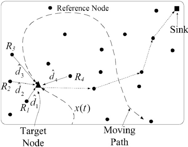
Figure 1. Wireless sensor network localization using UWB.
get node collects the coordinate information of reference nodes ,
, ,
, and
and denoted by dots, and their corresponding signal strength, by which to calculate the ranges between itself and the four reference nodes,
 ,
, ,
, and
and . Afterward, the target node derives its own coordinate, and sends to a sink, denoted by the square in Figure 1.
In order to enable communication between the target and reference nodes in the network, we assume that each and every node in the WSN is able to communicate through U-BOTH, proposed in this paper.
For convenience, the notation used in this paper is summarized in Table 1.

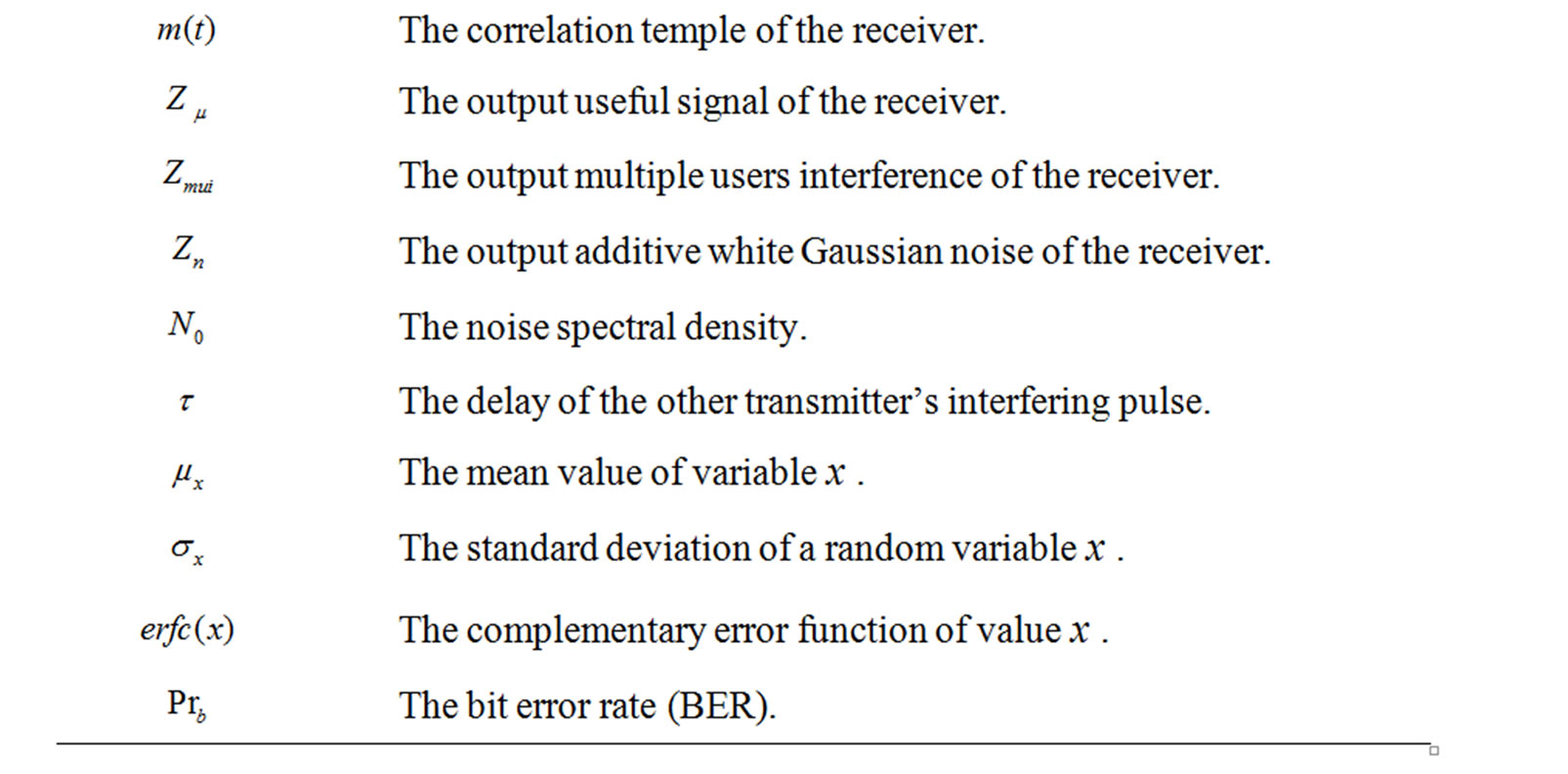
Table 1. Notation and meaning.
3. Physical Layer Model
3.1. UWB Signal Spreading and Modulation
First of all to achieve accurate localization in wireless communication, we need a reliable physical layer communication technique that reduces bit error rate (BER), while mitigating the multi-users-interference (MUI) and Gaussian noise interference. Our physical layer is a UWB system based on time-hopping (TH) signal transmission as well as OVSF (orthogonal variable spread factor) for spreading out the symbols.
OVSF (Orthogonal Variable Spread Factor) was extensively used in CDMA systems to provide variable spreading codes [19]. Shorter OVSF code lengths are usually optimized for short distance, high data rate transmission in less crowed environments due to its smaller spreading factor. On the other hand, time hopping (TH) is one of many signal modulation methods used by UWB. We will apply the time-hopping pulse position modulation (TH-PPM) algorithm to encode UWB pulse streams, and OVSF direct sequence to spread the user data bit stream, called U-BOTH (UWB modulation Based on OVSF and Time Hopping).
Figure 2 illustrates the utilization of time hopping (TH) pulse position modulation and OVSF spreading to encode a single bit in the user data stream. First, U-BOTH sends each bit in the bit time, denoted by . Then it modulates the bit 1 using a TH code, 12110021, in which each digit denotes a chip slot position within a frame time,
 , to send a broadband radio pulse. The number of pulses is denoted by
 . Therefore, each bit duration is
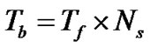 . Each chip slot lasts for
 , sufficient to send a short UWB pulse signal.
After the initial pulse position modulation using UWB signals, the pulse sequence is again applied with OVSF code so that the phases are shifted by![]() to provide orthogonality between multiple users. The length of the
to provide orthogonality between multiple users. The length of the
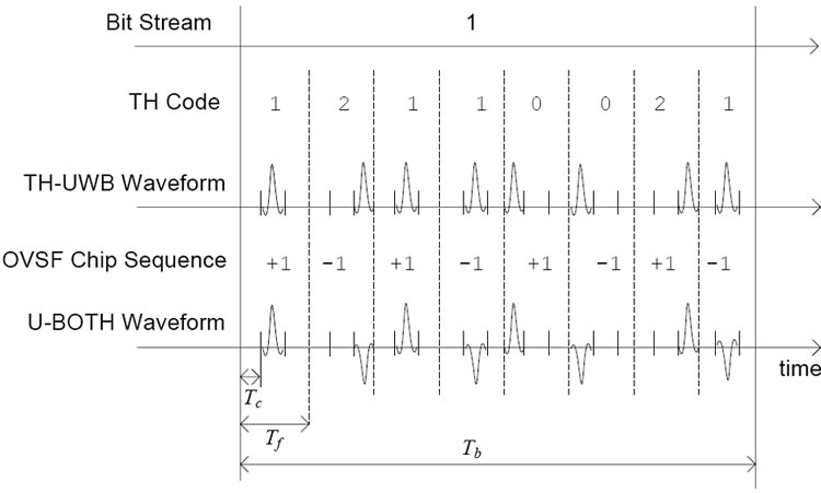
Figure 2. U-BOTH: Interference resistant UWB modulation using time hopping and OVSF.
OVSF code is called the spread factor SF, which is equal to .
.
In our system, the TH code is a pseudo-random sequence generated from foreknown seeds, such as node IDs. And the OVSF codes are selected from a welldefined set of orthogonal spreading codes.
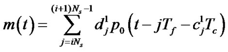
To formally analyze the system in this paper, we represent the transmitted signal by the nth transmitter in Equation (1):
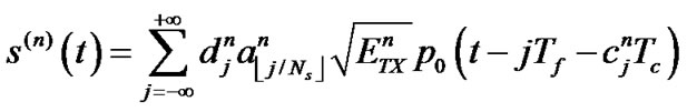 , (1)
, (1)
in which, is the OVSF code with the period
 ,
, is the energy of the n-th transmitter,
 is the energy normalized pulse waveform,
  is the TH code with period
 and
and indicates the data stream bit. If the data bit is 1,
 . Otherwise,
 .
.
At the receiver side, the received signal consists of three source of information:
 in which,
  is the desired user signal,
  is co-channel interference from multiple users, and
 is the additive white Gaussian noise (AWGN).
Denote the pulse energy of the n-th transmitter as .
.
Without loss of generality, we assume that the first user’s transmission is the desired signal at the receiver for simplicity, then Equation (2) provides the desired signal function at the receiver:
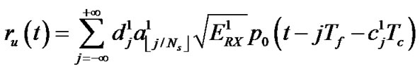 . (2)
. (2)
We define the correlation template of the receiver:
 ;
; . (3)
. (3)
3.2. Single User System Analysis
As the first step, we assume that the channel is the AWGN multipath-free channel, and that the transmitter and the receiver are synchronized. In a single user signal processing system, the input of the receiver has two parts:  and
and , and the output of the receiver in time interval [0, Tb] is represented by:
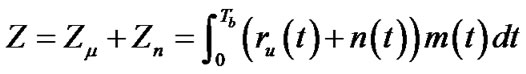 . (4)
. (4)
In Equation (4), the useful output signal is:
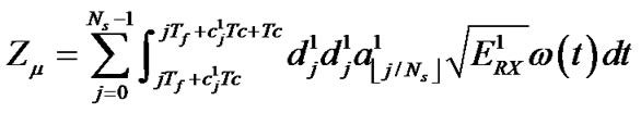 where
where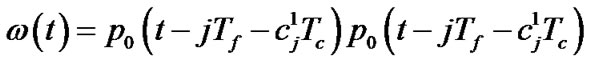 .
.
Because ,
, is the energy normalized pulse waveform, we have


 .
.
In Equation (4), the output noise signal is:
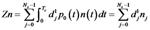 where
where is Gaussian random variable with mean 0 and variance
 . Because
 is not a random variable, the variance of
 is:
is:
 ,
,
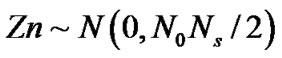 .
.
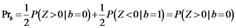
Suppose that the statistical probabilities of data bit b = 0 and b = 1 are equal, we obtain the BER (bit error rate) of the single user system in AWGN channel as follows:
 .
.
Because if b = 0, then the useful output is
 . Using Equation (4), the BER become:

 .
.
It can be rewritten by complementary error function  as follow:
 .
.
where .
.
Because U-BOTH is a rate variable system using OVSF, we analyze the relation between BER and the bit rate. Suppose the system’s OVSF code is a code tree of 6 layers [20], and the spreading factor is 2, 4, 8, 16, 32, 64, respectively. Further suppose the basic rate of our system is , then the corresponding bit rate of U-BOTH is
 (i = 32, 16, 8, 4, 2, 1, respectively).
Denote the bit rate as , where
 , i = 1, 2…32, we can get the relation between BER and the bit rate:
 , (5)
, (5)
Equation (5) shows that the BER decrease when the spreading factor SF increases or when the bit rate decreases. Therefore, we can adjust SF to adapt different environments with various noise levels while maintaining the same bandwidth of the signal. This is the main reason we adjust OVSF codes in our system.
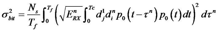
3.3. Multi-User Interference Analysis
In multi-user communication system, the received signal includes multi-user interference and noises. The
  part is the same as Equation (4), but the multi-user interference
 is additional. Because the phase and delay _ of interfering pulses is random as shown in Figure 3, we have to compute the interference’s variance.
Suppose that is uniformly distributed over [0,
 ), then the interference variance of the desired signal, i.e. the signal from the 1st user, caused by transmitter n is [14]:
 .
.
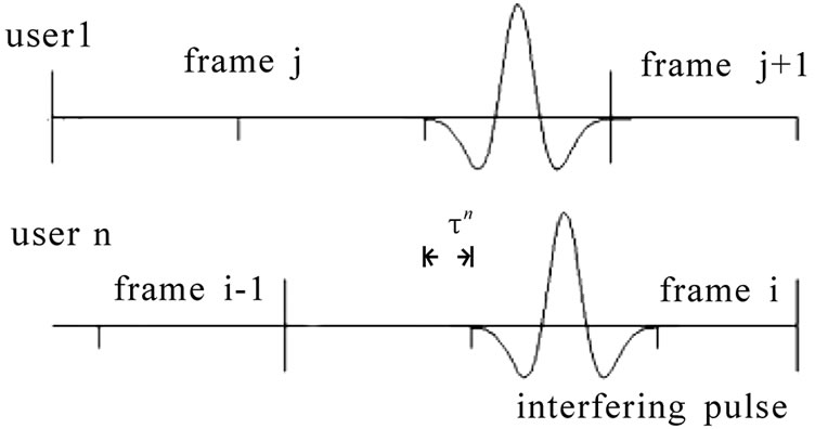
Figure 3. The Interference to User 1 by the n-th User.
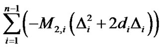
Therefore, the total interference variance from all other transmitters is:
 .
.
Because the delay![]() for all transmitters has the same distribution, we get the following formula:
for all transmitters has the same distribution, we get the following formula:
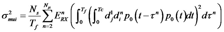
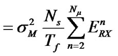 in which,
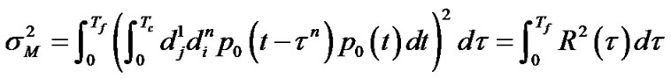 .
.
According to [14], and noticing that and
and  =
= =
= , Equation (6) gives the BER in multi-user interference environments.
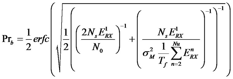
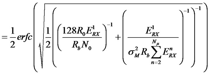 .
.
4. Network Protocol Operations
4.1. Protocol Operation
Our localization algorithms depend on a two-step process—the first step is for the target node to acquire the coordinate and signal strength information from reference nodes in the network using U-BOTH based communication protocols, and the second step is for the target node to calculate the distances to the reference nodes, and infer its own coordinate.
In order to get the necessary coordinate information from adjacent reference nodes, the following protocol steps are taken:
1) The mobile node broadcasts a location request message.
2) All the reference nodes send back packet with their own coordinates. During each short sampling period, a moving node can receive tens of responses from each of the reference nodes.
In wireless sensor networks, code assignments are categorized into transmitter-oriented, receiver-oriented or a per-link-oriented code assignment schemes (also known as TOCA, ROCA and POCA, respectively) [21, 22]. Depending on the ways of assigning the OVSF-TH codes and encoding the MAC data frames for transmissions, we propose two different ways to implement multiple access protocols using U-BOTH.
a) ROCA-Based Protocol Operations: The first approach is based on the receiver-oriented code assignment (ROCA), in which case the data packet transmissions are encoded using the unique OVSF-TH code assigned to the receiver. Beside ROCA, there is a common OVSF-TH code for bootstrapping and coordination purposes.
In ROCA scheme, when a target node needs to find out its coordinate, it sends a location request message using the common OVSF-TH code to the reference nodes. The request message includes the request command, and the receiver’s OVSF-TH code. Upon receiving the request message, each reference nodes sends back a response message using the receiver’s OVSF-TH code using a random backoff mechanism.
The response message includes each reference node’s identification information, and their coordinates.
b) TOCA-Based Protocol Operations: The second approach is based on transmitter-oriented code assignment
(TOCA), in which case each packet transmission is encoded using two OVSF-TH codes — one is a common OVSF-TH code to encode the common physical layer frame header, and the other transmitter-specific code is to encode the physical layer frame payload. The frame head includes the transmitter-oriented OVSF-TH code for encoding the frame payload.
Because the physical layer headers are sent on a common OVSF-TH code, the physical layer header transmissions resemble those of ALOHA networks with regard to packet collision. Because the headers are usually short, the collision probability is low.
On the other hand, because the data frame payload is transmitted on unique OVSF-TH codes, the interference between the payload and other frame headers and payloads is dramatically reduced.
In both ROCAand TOCA-based systems, packets from the reference nodes can be lost. However, this does not affect the overall performance of our localization algorithms because they tolerate such losses.
4.2. Location Calculation Algorithms
We make use of our OVSF-TH-UWB system and provide a UWB sensor localization network for mining applications to monitor environment and mineworker. We suppose moving nodes and other monitored nodes are the target nodes and every reference node knows its location. Suppose target node has a UWB RFID Tag equipped with transmitter and receiver to assist distributed localization with reference nodes. Data sink collect all the real-time localization information and send out to the monitoring center outside the mining area, as shown in Figure 1.
There are two steps in order to estimate the coordinate of the mobile node:
a) Ranging: Ranging is to estimate the approximate distance between the target node and the reference nodes. Target node estimates the distance from it to each reference node according to the RSSI values, using maximum likelihood estimation.
In this paper, we take ROCA scheme during ranging, target node broadcasts range-initiate (RI) packets for range estimates, and neighbor reference nodes reply with range-response (RR) packets, which include their coordinate and signal strength. To collect ranging and location information as much as possible in a short time, we take a dual-channel mechanism joint with common code and receiver code provided by OVSF-TH code. The receiver OVSF-TH code is generated by the unique MAC ID of receiver. Suppose target node i broadcast a RI packet via common channel code C0 at t = t1, and begin to listen the RR packets sent to its unique OVSF-TH code. This process initiate a window of time from t = t1 to t = t1 + Tw. The window-length Tw is much larger than RR duration TRR, which allows multiple RR gathered within window duration from adjacent reference nodes.
Following are the ranging and localization algorithm:
1) Target node i broadcasts RI packet at t = t1 on common code C0. This RI includes node i’s MAC ID and OVSFTH code Ci. When there is no interference, the RI arrives at a reference node j.
2) Reference node j delays after receiving the RI, and then reply a RR packet transmitted on the OVSF-TH code Ci. The RR packet includes node j’s MAC ID, transmitted signal strength and node i’s MAC ID. Where n is a random positive integer belong to [1, K], K is the average number of reference nodes in the transmitted range of target node. The delay
 is used to avoid interference between RR packets.
3) If t1 < t < t1 +Tw, node j continue to delay and then transmit RR packet via Ci.
4) Other reference nodes in the transmitted range of node i send RR packets by the same ways as node j in step 2 and 3.
5) If t = t1 + Tw, node i stop receiving RR packets.]
6) When t = t1 + Tw, node i received multiple RR packets from different reference nodes and several RR packets from the same reference node. It uses all the recorded information of PLi to estimates the distances to different reference nodes by MLE based RSSI ranging indicated in Equation (14) in Section 5.
b) Localization: Coordinate calculation, which is to determine the coordinate of the mobile node according to the coordinate information of the reference nodes and the corresponding distance from the target node to the reference nodes. Using the coordinates of the reference nodes and the estimated distance information, calculate the coordinate of the target node. It is implemented as follows:
1) When node i estimated all the distances to different reference nodes in its transmitted range, it applies these ranging results to Equation (15) in Section 6 and then computes its location based on the least squares algorithm.
2) When node i estimated its coordinate, it broadcasts ACK packet via its common channel code C0, informing finish of ranging. Its newest location is aware to neighbor nodes by the ACK and will arrive at the data sink through the localization routing.
According to above procedures of network protocol operations, after getting the reference coordinates and the respective signal strength information, a target node calculates its coordinate in two steps — ranging and localization. In order to fully take advantage of U-BOTH physical model in Section 3, we also design specific ranging algorithm and localization algorithm for U-BOTH in following sections.
5. Ranging Algorithm
Ranging is to estimate the approximate distance between the target node and the reference nodes. We use the maximum likelihood estimation for such calculations. First of all, we need to establish the path loss model of the UWB channel in order to inversely derive the distance information from received signal qualities.
5.1. The Path Loss Model
It is well-known that the path loss model can be expressed by the log-distance path loss law in many indoor or outdoor environments, as shown by Equation (7).
 ;
; , (7)
, (7)
in which
• d0 is the reference distance (e.g. 1 meter in UWB medium)
• PL0 means the path loss in dB at d0
• d is the distance between the transmitter (Tx) and receiver (Rx)
•  refers to the path loss exponent which depends on channel and environment
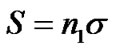
• S is the log-normal shadow fading in dB. Usually, S is a Gaussian-distributed random variable with zero mean and standard deviation![]() .
.
The tunnel’s environment in coal mine can be regarded as a special type of indoor environments, considering various kinds of concrete environmental factors in coal mine [17]. Thus, we adopt the UWB path loss model in coal mine based on residential indoor propagation model.
According to the residential indoor models, the values of ,
,![]() and S in Equation (7) are specific in each propagation environment, and could be treated as random variables [16].
and S in Equation (7) are specific in each propagation environment, and could be treated as random variables [16].
Accordingly, the UWB path loss is commonly modeled as:
 , (8)
, (8)
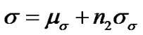
in which is the mean value of shadow fading’s standard deviation
 .
.
The probability density function (pdf) is:
 . (9)
. (9)
However, an unknown distance variable d appears in both the denominator and the exponent’s denominator in Equation (9), so it is hard to develop further statistical analysis. In addition, the path loss exponent in the aforementioned model is a random variable, and requires sufficient measurements on the spot in various residential environments before effectively being applied in generic scenarios. Especially, the standard deviation
![]() of the log-normal shadow fading S usually changes from locations to locations. Even if at the same location, it may change because of the time-varying channel. Thus, we need practical method to estimate S, especially for moving targets.
of the log-normal shadow fading S usually changes from locations to locations. Even if at the same location, it may change because of the time-varying channel. Thus, we need practical method to estimate S, especially for moving targets.
Therefore, in order to apply above path loss model, IEEE 802.15.4a Task Group provided Channel Model 1-9 by taking limited real measurements to determine the values of ,
,![]() and other variables in different situations. When deploying real UWB networks, people could approximately choose the corresponding channel model with the parameters specified in IEEE 802.15.4a.
and other variables in different situations. When deploying real UWB networks, people could approximately choose the corresponding channel model with the parameters specified in IEEE 802.15.4a.
We propose a UWB coal mine propagation model based on many other modeling methods for the application of ranging and localization. In this model, the mean value of the path loss exponent is given for different tunnel environments, and the log-normal shadow fading S is represented through a random variable as follows:
 .
.
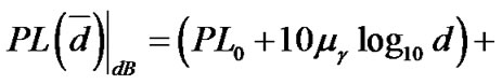
Then, the indoor UWB path loss could be expressed as:
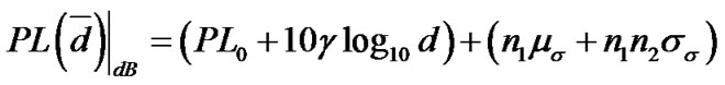 , (10)
according to Equation (7).
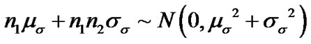
In Equation (10),  and
and are zero-mean Gaussian variables of unit standard deviation,
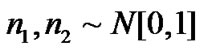 . (PL0+10 log10 d) is the median path loss, and
 represents the random variation about the median path loss. According to the “3
![]() principle” in Gaussian distribution, the probability of a Gaussian variable lying in the range
principle” in Gaussian distribution, the probability of a Gaussian variable lying in the range is 99.73%, even though the range of Gaussian random variable is
 . That is, 99.73% value of variables
 and
and is within the range of (-3, +3). Furthermore, it dramatically simplifies computation if we use truncated Gaussian distributions for
 and
and so as to keep
 and
and ![]() from taking on impractical values. According to [16], we confine
from taking on impractical values. According to [16], we confine , and
, and .
.
In aforementioned model,  is not exactly Gaussian because
 is not Gaussian variable. However, the product is very small with respect to whole expression of path loss. Thus, the path loss PL(d) is approximately a Gaussian-distributed random variable with:
 ,
,
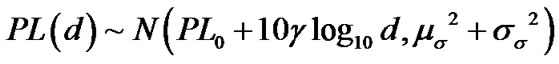 .
.
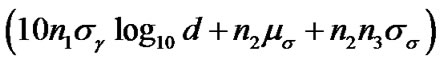
The probability density function (pdf) of the path loss PL(d) is:
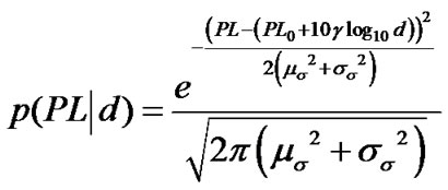 . (11)
Compared with the model in [16], our UWB coal mine propagation model given by Equation (11) is more convenient to carry out parameter estimation and statistic analysis because it simplifies the statistics and PDF. What is more, when considering the random influence of the log-normal shadow fading, this model is generic than current models in IEEE 802.15.4a.
5.2. Ranging Algorithm Based on Maximum Likelihood Estimation
The distance between the transmitter Tx and the receiver Rx in Equation (10) can be calculated by the general ranging method between two nodes using the RSSI information:
Receiver computes the distance between the transmitter Tx and the receiver Rx using random values and
and  in the truncated range. This method takes into account the influence of real log-normal shadow fading on raning and decreases the ranging error compared to the models in IEEE 802.15.4a.
However, the random variables and
and selected by the transmitter Tx are not exactly those in the real time-variant channel. In order to avoid the ranging errors caused by the large deviation between the simulated
  and
and values and the real
 and
and values in each round of ranging estimation, we propose an iterative ranging based on MLE (maximum likelihood estimation) in UWB wireless sensor networks.
Suppose PLi is the ith observation value, we get the joint conditional pdf  using Equation (12).
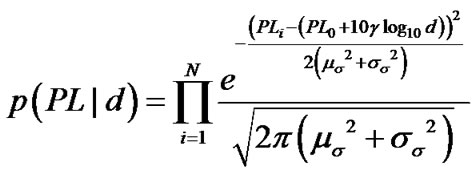 . (12)
The necessary condition to compute the MLE of d is:

 . (13)
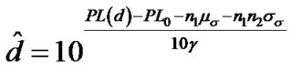
We solve Equation (13) and have:
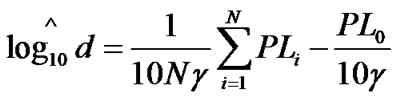 .
.
Therefore, the MLE based RSSI UWB ranging is:
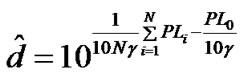 . (14)
6. Localization Algorithm
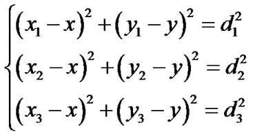
When computing the location of a wireless sensor node, there are two types of nodes, the reference node and the target node. Suppose that we have three reference nodes with coordinates ,
, and
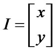
and , respectively. The target node computes its coordinate
 using trilateration method with the coordinates of reference nodes and their ranges
 , to the target node using the following equations:
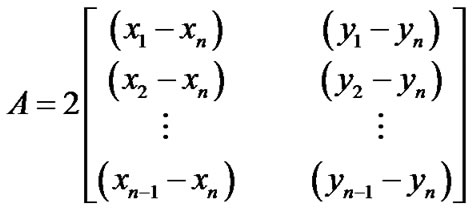
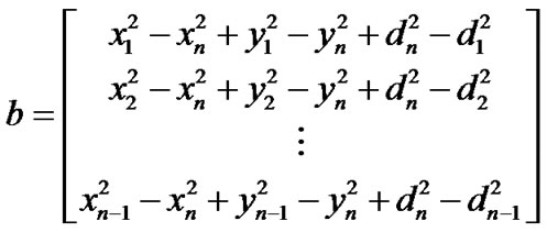
In practical situations, three reference nodes are usually insufficient to accurately derive the target coordinate due to ranging errors from thermal noise and other interferences. The least squares algorithm uses multiple reference nodes and the corresponding ranges to improve accuracy in the presence of error. It first creates following equations:
 (15)
(15)
where and
and (i = 1,2,…,n)are the coordinate of the reference nodes, and the distances to the target node.
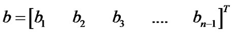
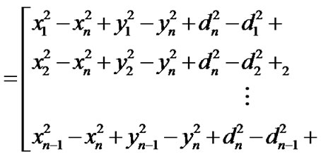
These equations can be linearized by subtracting the last low and performing some minor arithmetic shuffling, resulting in the following relations AI = b:
 ,
,
 ,
,
 .
.
This work employs the following solution:
 . (16)
Although the least squares algorithm could reduce the localization error, it requires a large amount of reference nodes within the communication radius of target node. Therefore, in the mining application of UWB wireless sensor networks, it is necessary to balance the cost and the accuracy.
In the following, we explore the relation between localization error and ranging error and then propose a modified algorithm based on the least squares algorithm.
Assume that the estimated distance between the target node and the ith reference node is , where
  is the ranging error,
 . From Equation (16), we have
 , where

 ,
,
 .
.
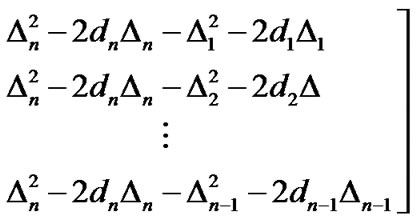
Denote , we get the coordinate
  of target node:
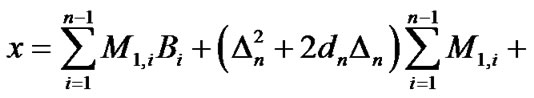
 .
.

 . (18)
Usually, , and are mutually independent. Therefore,
 . (19)

 . (20)
From above deduction, it is shown that localization error could be reduced proportionally to the reduction in the ranging error. According to the relation, if we guarantee the accuracy of in every equation, the trilateration and the least squares algorithm could be kept similarly accurate even if the number of equations is limited. The proposed ranging solution using MLE based on RSSI in this paper improves the ranging accuracy between target node and every reference node through iterative ranging, and reduces the ranging error caused by ranging based on a single round sampling. Furthermore, it reduces the influence of fixed value of
 given in our path loss model on ranging and localization in timevariant channel. Hence, our localization algorithm can provide accurate ranging and localization with less UWB reference nodes.
7. Simulation Results
In order to verify our localization algorithms based on U-BOTH system for WSNs, we carried out simulation in the following scenarios:
1) With regard to the BER (bit error rate), we evaluate U-BOTH system performance in single and multi-user scenarios.
2) Using the sample network deployment as shown in Figure 4, we evaluate the ranging accuracy by comparing the results with the Cramer-Rao lower bounds.
3) Using the same sample network as shown in Figure 4, we evaluate the impact of the number of itera-
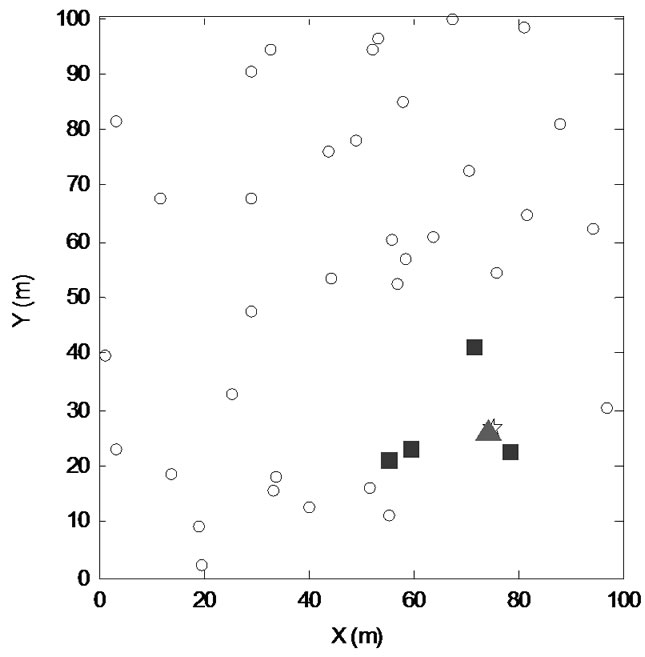
Figure 4. Wireless sensor network simulation for localization.
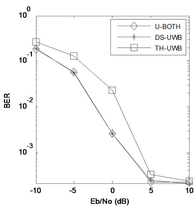
Figure 5. Bit error rate in a single user system with additive white Gaussian noise (AWGN).
tions in calculating the coordinate of a specific target node, indicated by the triangle in the diagram.
7.1. U-BOTH System Performance
We assume the channel is AWGN multipath-free single user channel; the transmitter and the receiver are synchronized perfectly. Then we randomly generate 2000 bits, every bit uses 4 pulses to repeat coding (Ns = 4).
Figure 5 illustrates the BER of the received signal using U-BOTH system, in contrast to DS-UWB that only uses direct sequence spreading, and TH-UWB that uses time-hopping pulse position modulation alone for UWB transmissions. We can see that the BER of U-BOTH and the DS-UWB system which use the![]() -phase shift keying modulation are lower than TH-UWB. This is because the distance of two signals in binary phase shift keying (BPSK) modulation is
-phase shift keying modulation are lower than TH-UWB. This is because the distance of two signals in binary phase shift keying (BPSK) modulation is , but
, but 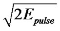 in THUWB [23].
Secondly, we let Eb = N0 = 0 dB, Ns = 4 and generated 2000 bits randomly. Figure 6 shows the relative performance of U-BOTH, TH-UWB and DS-UWB systems in multiple access scenarios. In this case, the received signal includes by noise and co-channel interference. In Figure 6, although both the BER and the variance of error bits increase as the number of users increases, the performance of our U-BOTH system is still better than DS-UWB and TH-UWB, proving that the UWB coding based OVSF-TH effectively handle the burst errors.
7.2. Evaluation of the Ranging Algorithms
In order to evaluate the performance of the ranging algorithms, we compare the parameter estimation errors against the Cramer-Rao lower bound (CRLB).
Denote![]() as the unbiased estimation of the parameter d from Equation (13), then the mean square error (MSE) of
as the unbiased estimation of the parameter d from Equation (13), then the mean square error (MSE) of![]() is
is
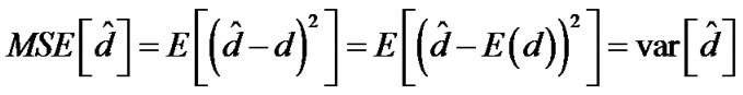 . (21)
Hence in unbiased condition, the MSE of![]() is equal to the variance. The lower bound of the MSE based on UWB RSSI ranging could be represented by the CRLB:
is equal to the variance. The lower bound of the MSE based on UWB RSSI ranging could be represented by the CRLB:
 .
.
From Equation (13), we know that can
can
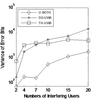
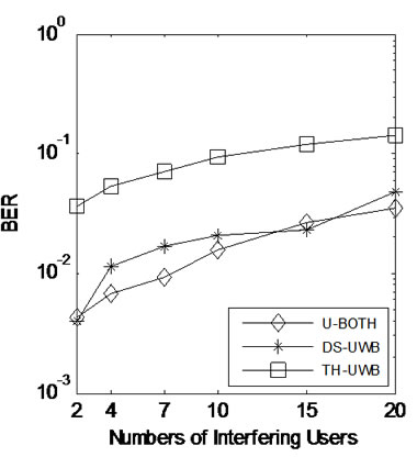
Figure 6. Bit error rate and the variance of the number of error bits of 2000 generated bits.
not be expressed in the form . So, the lower bound of MSE can not reach the CRLB. However, we can use the MLE based RSSI ranging to enable the MSE to approach the CRLB. The MSE of UWB ranging is:
 . (22)
As PLi are mutually independent, we take Equation (12) and Equation (14) into Equation (22), and get the MSE of MLE based ranging using RSSI information:
 .
.
Therefore, the MSE of estimated distance![]() is the function of real distance d and the number of iterations N.
is the function of real distance d and the number of iterations N.
Based on the data in [7,11,16], we set n1, n2 Î [-2, 2], n1n2Î [-4, 4] and adopt values of UWB path loss model for simulations as shown in Table 2.
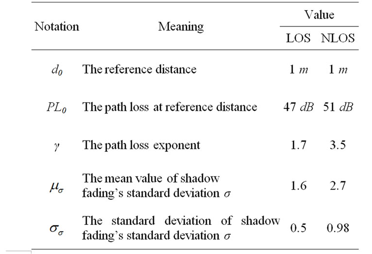
Table 2. Portion of the simulation parameters.

Figure 7. comparisons between the cramer-rao lower bound (crlb) and the mean square error (mse) of ranging estimations at different distances.

Figure 8. Comparisons between the cramer-rao lower bound (CRLB) and the mean square error (MSE) of ranging estimations, regarding the number of iterations N.

Figure 9. The impact of the number of iteration n to the ranging errors at different distances.
Figure 7 illustrates the relation between d and the CRLB, and the relation between d and the MSE. On one hand, it shows that the CRLB and the MSE increase when d increases, on the other, the MSE of ranging and the CRLB are always very close. When d is very small, they even overlap with one another. The more iterations we have for ranging, the smaller difference between the CRLB and the MSE (When d = 4m, N = 20, the CRLB is 0.0412m2, the corresponding MSE is 0.0414m2. When d = 20m, N = 20, the CRLB is 1.0310 m2, the corresponding MSE is 1.0357 m2).
In Figure 7, we can see that when N = 20, d > 20m, the MSE of ranging estimation grows higher than 1m2. Therefore, it is necessary to filter out large d values in order to achieve higher ranging accuracy.
In the MLE based ranging using the RSSI values, the number of iterations N is an important parameter. Figure 8 gives the relation between N and the CRLB and the MSE, respectively. When N increases, the CRLB and the MSE decrease rapidly. The MSE of ranging approximates the CRLB when N is large enough (e.g. when d = 5m, N = 10, the CRLB is 0.1289 m2, the corresponding MSE is 0.1300 m2). Accordingly, we validate Equation (23), and prove the validity of our MLE method.
Figure 9 compares the MLE based ranging errors when the numbers of iterations N are 1, 5, and 20. Even if thermal noises and other interferences cause the error to fluctuate randomly, we can see that higher numbers of iterations dramatically increase the accuracy of ranging computations.
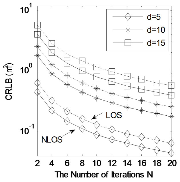
Figure 10. The cramer-rao lower bound (crlb) of ranging estimations in los (line of sight) and nlos (non-line of sight) environments.

Figure 11. Realtion between the mean square error (MSE) of ranging estimation and the localization error.
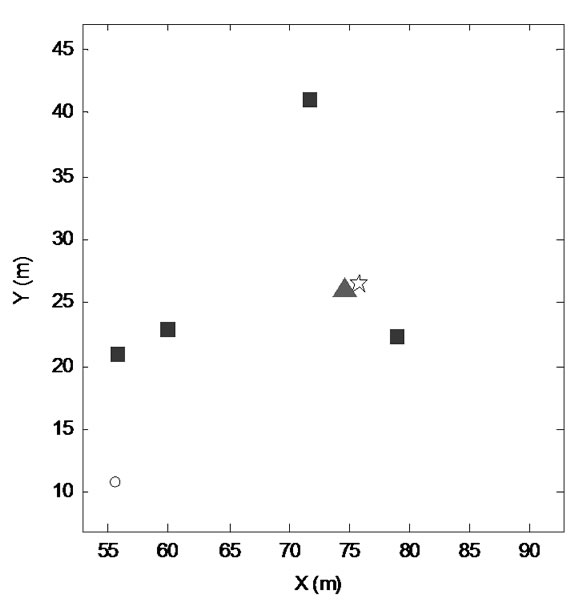
Figure 12. Localization result of estimation time N=1 (localization error is 1.2547m).
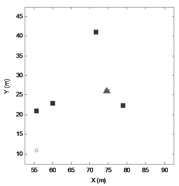
Figure 13. Localization result of estimation time N=20 (localization error is 0.2464m).

Figure 14. Localization result of estimation time N= 100 (localization error is 0.0885m).
Figure 10 analyzes the CRLB, which reflects the MSE of unbiased estimation, in LOS (line of sight) and NLOS (non-line of sight) environments. When N increases, the CRLB in LOS and NLOS decrease correspondingly. For the same distance d situations, the CRLB in NLOS is even smaller than the CRLB in LOS through our channel model and ranging method. Therefore, precise ranging and localization estimation also could be achieved in NLOS environment. This is especially attractive in coal mine environments.
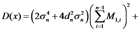
7.3. Evaluation of the Localization Algorithms
From the analysis of Cramer-Rao low bound in Equation (21), the variance of ranging error can be shown in Equation (23). Similarly, the localization error can be expressed by the estimated coordinates and the real coordinates as .
.
Figure 11 shows the relation between ranging error and localization error in Equation (19) and Equation (20). It is obvious that the ranging error and localization error decrease when N increases. The localization error when N = 2 is about 2/3 of that when N = 1. When N = 20, we could get the least localization error, which is 0.3009m.
Secondly, we choose some nodes in Figure 4 to examine the impact of the number of iterations to the accuracy of localization computations as shown in Figure 12, Figure 13 and Figure 14. The triangle is the target node, the squares are reference nodes in the communication radius of the target node, the star is the estimated location of target node and the hollow circles are other nodes. We set the communication radius in Figure 4 to be 20m, and the average number of reference nodes in this range to be K = 5. Therefore, allocating about 40 reference nodes in the mining area should be enough to monitor target node. As the location calculation algorithms described in Section 4-B, when Tw = 1s, TRR = 10ms and
 = 10ms, we can ensure 20 to 100 rangings between target node and every reference node. Figure 12, 13, 14 display the special deviation between estimated location and real location when N = 1, N = 20 and N = 100. Table 3 shows the localization error between the target node and a reference node that is d = 14.9430m away, which shows that the impact of N increments decreases when N is greater than a few dozen.
8. Conclusions
We proposed a group of communication protocols and localization algorithms for wireless sensor networks in coal mine environments, namely a new UWB coding method, called U-BOTH (UWB based on Orthogonal Variable Spreading Factor and Time Hopping), an ALOHA-type channel access method and a message exchange protocol to collect location information. Then we derived the corresponding UWB path loss model in order to apply the maximum likelihood estimation (MLE) method to compute the distances to the reference sensors using the RSSI information, and provided least squares (LS) method to estimate the coordinate of the moving target. The performance of U-BOTH communication system and the localization algorithms are analyzed using communication theories and simulations. Results show that UBOTH transmission technique can effectively reduce the bit error rate under the path loss model, and the corresponding ranging and localization algorithms can accurately compute moving object locations in coal mine environments.
9. Acknowledgment
We would like to express our sincere appreciation to Prof. Fanzi Zeng, and Prof. Juan Luo for their insightful feedbacks during the preparation of this manuscript, and of the anonymous reviewers for their helpful comments. This work has been generously sponsored in parts by the National Natural Science Foundation of China under Grant No. 60673061 and the Raytheon Company under Grant No. RC-42621.

Table 3. The impact of the number of interations N to the localization errors when distance d = 14.9430m.
10. References
[1] T. A. Alhmiedat and S. H. Yang, “A survey: Localization and tracking mobile targets through wireless sensors network,” In The Eighth Annual PostGraduate Symposium on the Convergence of Telecommunications, Networking and Broadcasting (PGNET), 2007.
[2] N. Patwari, A. O. Hero, M. Perkins, N. S. Correal, and R. J. O’Dea, “Relative location estimation in wireless sensor networks,” IEEE Transactions on Signal Processing, Vol. 51, pp. 2137, 2003.
[3] P. Bahl and V. Padmanabhan, “RADAR: An in-building RF-based user location and tracking system,” In INFOCOM, 2000.
[4] K. Whitehouse and D. Culler, “Macro-calibration in sensor/actuator networks,” In Mobile Networks and Applications (MONET), Vol. 8, pp. 463–472, 2003.
[5] T. He, J. A. Stankovic, C. Huang, T. Abdelzaher, and B. M. Blum, “Range-free localization schemes for large scale sensor networks,” In Proceedings of the Annual International Conference on Mobile Computing and Networking (MOBICOM), pp. 81–95, 2003.
[6] IEEE Std 802.15.4a. part 15.4a, “Low rate alternative PHY task group (TG4a) for wireless personal area networks (WPANs),” Technical Report, IEEE, June 2007.
[7] A. F. Molisch, D. Cassioli, and C. -C. Chong, “A comprehensive standardized model for ultrawideband propagation channels,” IEEE Transactions on Antennas and Propagation, Vol. 54, No. 11, pp. 3151–3166, 2006.
[8] I. Bucaille and A. Tonnerre, “MAC layer design for UWB LDR systems: PULSERS proposal,” In 4th Workshop on Positioning, Navigation and Communication (WPNC), pp. 277–283, 2007.
[9] A. Fujii and H. Sekiguchi, “Impulse radio UWB positioning system,” In IEEE Radio and Wireless Symposium, pp. 55–58, 2007.
[10] L. D. Nardis and M.-G. D. Benedetto, “Positioning accuracy in ultra wide band low data rate networks of uncoordinated terminals,” In IEEE International Conference on UWB (ICUWB), pp. 611–616, 2006.
[11] S. Venkatesh and R. M. Buehrer, “Multiple-access design for Ad Hoc UWB position-location networks,” In Proceedings IEEE Wireless Communications and Networking Conference (WCNC), Vol. 4, pp. 1866–1873, 2006.
[12] Y. Wang, Z. Wang, and H. Yu, “Simulation study and probe on UWB wireless communication in underground coal mine,” Journal of China University Of Mining and Technology (English Edition), Vol. 16, No. 3, pp. 296– 300, 2006.
[13] M. Z. Win and R. A. Scholtz, “Ultra-wide bandwidth time-hopping spread-spectrum impulse radio for wireless multiple-access communication,” IEEE Transaction on Communication, Vol. 48, No. 4, pp. 679–691, 2000.
[14] M. G. D. Benedetto, and G. Giancola, “Understanding ultra wide band radio fundamentals,” Prentice Hall, New Jersey, 2004.
[15] T. Gigl and G. J. M. Janssen, “Analysis of a UWB indoor positioning system based on received signal strength,” In 4th Workshop on Positioning, Navigation and Communication (WPNC), pp. 97–101, 2007.
[16] S. S. Ghassemzadeh, R. Jana, C. W. Rice, W. Turin, and V. Tarokh, “Measurement and modeling of an ultra-wide bandwidth indoor channel,” IEEE Transaction on Communication,Vol. 52, No. 10, pp. 1786–1796, 2004.
[17] F. Li, P. Han, X. Wu, and W. Xu, “Research of UWB signal propagation attenuation model in coal mine,” Lecture Notes in Computer Science, Vol. 4611, pp. 819–828, 2007.
[18] C. Savarese, J.M. Rabaey, and J. Beutel, “Locationing in distributed Ad-Hoc wireless sensor networks,” In Proceedings IEEE International Conference on Acoustics, Speech, and Signal, Vol. 4, pp. 2037–2040, 2001.
[19] F. Adachi, M. Sawahashi, and K. Okawa, “Tree-structured generation of orthogonal spreading codes with dierent lengths for the forward link of DS-CDMA mobile radio,” IEE Electronics Letters, Vol. 1, No. 1, pp. 27–28, January 1997.
[20] H. Cam, “Nonblocking OVSF codes and enhancing network capacity for 3G wireless and beyond systems,” Special Issue of Computer Communications on 3G Wireless and Beyond for Computer Communications, Vol. 26, No. 17, pp. 1907–1917, 2003.
[21] M. Joang and I. T. Lu, “Spread spectrum medium access protocol with collision avoidance in mobile ad-hoc wireless network,” In Proceedings of IEEE Conference on Computer Communications (INFOCOM), pp. 776–83, New York, NY, USA, March 21-25, 1999.
[22] T. Makansi, “Trasmitter-oriented code assignment for multihop radio net-works,” IEEE Transactions on Communications, Vol. 35, No. 12, pp. 1379–82, December 1987.
[23] J. G. proakis, Digital communications: Fourth Edition, McGrawHill, Columbus, 2001
NOTES
* This work was sponsored in parts by the National Natural Science Foundation of China under Grant No. 60673061 and the Raytheon Company under Grant No. RC-42621.