Journal of Electromagnetic Analysis and Applications
Vol. 1 No. 4 (2009) , Article ID: 1122 , 10 pages DOI:10.4236/jemaa.2009.14041
A Novel PSO Algorithm for Optimal Production Cost of the Power Producers with Transient Stability Constraints
![]()
1Department of Electrical Engineering, Annamalai University, Annamalainagar, Tamil Nadu, India, 2Department of Electrical & Electronics Engineering, Pondicherry Engineering College, Puducherry, India.
Email: vishanitha@yahoo.com
Received April 29th, 2009; revised July 10th, 2009; accepted July 23rd, 2009.
Keywords: Optimal Power Flow, Production Cost, Ramping Cost, Fitness Distance Ratio Particle Swarm Optimization, Transient Stability Limit, Piecewise Linear Ramp Rate Limit
ABSTRACT
The application of a novel Particle Swarm Optimization (PSO) method called Fitness Distance Ratio PSO (FDR PSO) algorithm is described in this paper to determine the optimal power dispatch of the Independent Power Producers (IPP) with linear ramp model and transient stability constraints of the power producers. Generally the power producers must respond quickly to the changes in load and wheeling transactions. Moreover, it becomes necessary for the power producers to reschedule their power generation beyond their power limits to meet vulnerable situations like credible contingency and increase in load conditions. During this process, the ramping cost is incurred if they violate their permissible elastic limits. In this paper, optimal production costs of the power producers are computed with stepwise and piecewise linear ramp rate limits. Transient stability limits of the power producers are also considered as additional rotor angle inequality constraints while solving the Optimal Power Flow (OPF) problem. The proposed algorithm is demonstrated on practical 10 bus and 26 bus systems and the results are compared with other optimization methods.
1. Introduction
The electric power industry is restructured around the world to meet the growing load demand. In the restructured power market, most of the power transfer is carried out through wheeling transactions [1]. Power system planners and operators often use Optimal Power Flow (OPF) as a powerful assistant tool in both planning and operating stage. OPF problem is aimed to optimize the operating cost of the power system while satisfying various system operating constraints. Due to the nonlinear nature of the problem, many researchers explored the artificial intelligence techniques to have the minimum solution [1–4].
Though OPF problem minimizes the cost while satisfying the practical constraints like line flow, voltage limits etc., it has to satisfy the stability limits also. Due to the competitive expansion in recent years, power system operation has become highly stressed, unpredictable and vulnerable [5]. A stressed system has more contingencies and become more vulnerable. Due to the occurrence of large blackouts, stability constraints are inevitable while solving the optimal power flow problem [6]. Many researchers have solved the transient stability constrained OPF problem using various methods [7–12].
In the real time power market, the critical contingencies and sudden load changes forced the operation of the Independent Power Producers (IPPs) beyond their operating power limits. But the operations are restricted by their ramp rate limits. When the operating range of the generator is within the elastic range of the strength of the shaft, the corresponding ramping process will not shorten the life of the rotor and no ramping costs are incurred. When it violates the elastic range, the economic impact due to rotor fatigue is expressed in terms of the ramping cost [13] and the authors argued that the ramping costs should be incorporated into the system operation costs.
Shrestha et al. derived the operating cost of the power producers by considering ramping rate and time with conventional quadratic cost function [14]. Tanaka described an extended form of real time pricing that achieves the optimal rate of change in demanded quantity by considering the ramping costs into account. The steepness of the load curve is controlled by the proposed optimal pricing policy, which reduces the ramping cost and the possibility of large scale blackout [15].
In the above literature, fixed ramping rate limits are used to incur the cost with respect to the contingencies and system fluctuations. But the strict ramping rate of the power producers will increase the production cost and hence the stepwise ramping rate [16] has been proposed. But in reality the dispatch schedules of the independent system operators have not been executed by the power producers due to the restricted ramping period [17,18]. Hence the piecewise linear ramping model was proposed by Shahidehpour et al. [19] to solve unit commitment problem and find their applications in the operation of Independent System Operators [17,18].
Conventional methods like lambda iteration method offer good results but when the search space is non linear and has discontinuities like piecewise linear ramping, these methods become difficult to solve with a slow convergence ratio and not always seeking to the global optimal solution. Hence, Optimal Power Flow problem considered in this paper is solved using a novel Fitness Distance Ratio based swarm algorithm with transient stability limit. The power producers adjust their operating points when the system is subjected to credible contingencies and sudden load variations. If the change in power output of the power producers violates their permissible limits, the ramping cost is computed. A linear ramping model is validated to compute the ramping cost of the power producers with a utility test system.
2. Problem Formulation
Optimization of production cost function F of generation has been formulated based on classical OPF problem with line flow constraints. For a given power system network, the optimization of production cost of generation is given by the following equation.
F = Min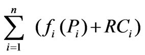 $ / h(1)
where F is the total operating cost of power producers, fi (Pi) is the fuel cost of the ith power producer. RCi is the ramping cost of the power producer and n is the total number of power producers connected in the network.
The fuel cost function of the ith generator is given by fi (Pi) = a0 + a1 Pi + a2 Pi2 $ / h (2)
where Pi is the real power output of an ith power producer and a0, a1, a2 are the fuel cost coefficients of the ith power producer.
Ramping cost is considered to be negligible when the power producers operate within the limits. However, strict ramping limits restrict their operation. If they are permitted to extend their limits, the life of the rotor will be affected. Hence the operation beyond the safe limits is charged as ramping cost. This ramping cost is cumulated with the fuel cost which is termed as production cost of the power producers.
Even though, the ramping actions of the power producers are governed by limits, they change their operating states with respect to time. Figure 1 shows the variation of output during the ramping process. It consists of piecewise linear ramping period [0, RTm] and a constant output period [RTm, 1 h].
The power output of the power producer during the first interval between (0, RT1) is given by Pi = 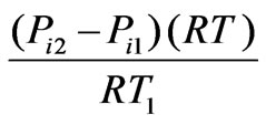 + Pi1 (3)
where RT is the total ramping time of the power producer.
Similarly, the power output of the power producer during the second interval between (RT1 , RT2) is given by Pi = 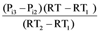 + Pi2
+ Pi2
In general, the power output of the power producer in any interval among the m segments during the linear ramping period (0, RTm) is given as follows:
Pi =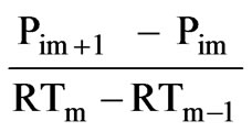 (RT – RT (m -1))+ Pim , 0
m is segment index The power output of the power producer during the constant output period between the interval (RTm ,1) is given by
Pi = Pi + RR * RT, RTm< RT <1(5)
where RR is the ramping (up/down) rate and RT is the ramping time of the ith power producer.
The above formulation includes the m linear segment regions before the power producers obtain its ramping limit in the specified time interval. This formulation is
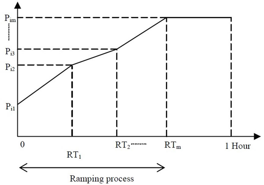
Figure 1. Power delivery during a time interval
used to compute the ramping cost of the power producers at their corresponding operating point. This information is followed by the ISOs [17,18] during the rescheduling process of the power producers at the insecure conditions.
When the ramping process is included in the power dispatch, the effective operating cost of a unit considering the change of the power output is given by F = 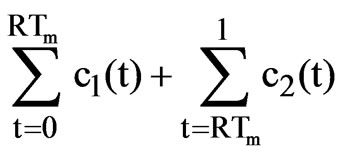 (6)
(6)
where c1(t) is the optimal production cost between the interval 0 and RTm and is given by c1(t) =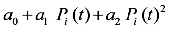 , t Î (0, RTm)
where Pi(t) =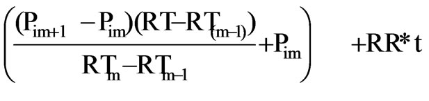 ,
,  (7)
(7)
c2(t) is the optimal production cost between the interval RTm and 1 and is given by c2(t) = a0 + a1Pi(t) + a2Pi(t)2, t Î (RTm , 1)
where Pi(t) = Pi + RR* RT(8)
In the above expressions, the term RR represents either increase ramp rate (UR) or decrease ramp rate (DR). When the power producers are operating beyond their permissible limits, ramping cost is calculated using the above formulation.
The operating cost function of the power producer given in the equation 1 is subjected to the following constraints.
* – PL – PD = 0(9)
where PD is the total load of the system and PL is the transmission losses of the system.
* The inequality constraint on real power generation Pi of each power producer i is given by Pimin £ Pi £ Pimax(10)
* Power limit on transmission line is given by MVAfp,q £ MVAfp,qmax(11)
where MVAfp,qmax is the maximum rating of transmission line connecting buses p and q.
* Transient stability constraint is expressed in terms of generator rotor angles which are given as follows:
dmin £ di £ dmax(12)
where di is the relative rotor angle of the ith power producer with respect to the reference.
3. Overview of Particle Swarm Optimization
Kennedy and Eberhart first introduced the PSO method which is motivated by social behavior of organisms such as fish schooling and birds flocking [20]. In a PSO system, particles fly around a ‘d’ dimensional problem space. During flight, each particle adjusts its position according to its own experience as well as by the best experiences of other neighboring particles. Let us consider Xi = (Xi1, Xi2 … Xid) and Vi = (Vi1, Vi2 … Vid) be the position and velocity of the ith particle. Velocity Vid is bounded between its lower and upper limits. The best previous position of the ith particle is recorded and is given by Pbesti = (Pi1, Pi2, … Pid ). Let gbesti = (Pg1, Pg2, … Pgid) be the best position among all individual best positions achieved so far. Each particle’s velocity and position is updated using the following two equations.
Vidk+1=W*Vidk+C1*rand1*(Pid–Xid)+C2*rand2*(Pgid –Xid)(13)
Xidk+1 = Xidk + Vidk+1 (14)
where C1 and C2 are the acceleration constants, which represent the weighting of stochastic acceleration terms that pull each particle towards Pbest and gbest positions. K represents the current iteration and rand1 and rand2 are two random numbers in the range zero to one. Inertia weight W is a control parameter that is used to control the impact of the previous velocities on the current one. Hence, it influences the trade-off between the global and local exploration abilities of the particles. The search process will terminate if the number of iterations reaches the maximum allowable number.
4. FDR PSO Algorithm
In the literature, it has been reported that the particle positions in PSO oscillate in damped sinusoidal waves until they converge to points in between their previous Pbest and gbest positions [21,22]. During this oscillation, if a particle reaches a point, which has better fitness than its previous best position, then the particle continues to move towards the convergence of the global best position discovered so far. All the particles follow the same behavior to converge quickly to a good local optimum. Suppose, if the global optimum of the problem does not lie on a path between original particle positions and such a local optimum, then the particle is prevented from effective search for the global value. In such case, many of the particles are wasting their computational effort in seeking to move towards the local optimum already discovered. Better results may be obtained if various particles explore other possible search directions.
In the FDR PSO algorithm, in addition to the Sociocognitive learning processes, each particle also learns from the experience of neighboring particles that have a better fitness than itself [23]. The implementation of this idea is simple based on computing and maximizing the relative fitness distance ratio. The proposed algorithm does not introduce any complex computations in the original PSO algorithm.
This approach results in change in the velocity update equation, although the position update equation remains unchanged. It selects only one other particle at a time when updating each velocity dimension and that particle is chosen to satisfy the following two criteria.
1) It must be near the current particle.
2) It should have visited a position of higher fitness.
The simplest way to select a nearby particle which satisfies the above mentioned two criteria is that maximizes the ratio of the fitness difference to the one-dimensional distance. In other words, the dth dimension of the ith particle’s velocity is updated using a particle called the nbest , with prior best position Pj. It is necessary to maximize the following Fitness Distance Ratio which is given by
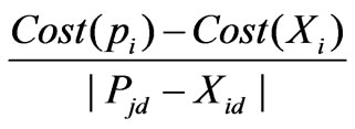 (15)
(15)
In the FDR PSO algorithm, the particle’s velocity update is influenced by the following three factors:
1) Previous best experience i.e. Pbest of the particle
2) Best global experience i.e. gbest , considering the best P best of all particles.
3) Previous best experience of the “ best nearest” neighbor i.e. nbest.
Hence, the new velocity update equation becomes:
Vi dk+1=W*Vidk + C1*rand1*(Pid–Xid)+C2*rand2* (Pgid – Xid) +C3 *rand3 (Pnd - Xid)(16)
where Pnd is the nearby particle that have better fitness.
The position update equation remains the same as in Equation (13).
The overall evolution of the PSO and FDR PSO population resembles that of other evolutionary algorithms. The main difference is that algorithms in the PSO family retain historical information regarding points in the search space already visited by the various particles, this is a feature not shared by other evolutionary algorithms.
PSO algorithm performs well in initial iterations but fails to make further progress in later iterations as the population diversity is rapidly lost. Hence PSO algorithm suffers from premature convergence in many applications. But in FDR PSO algorithm, the average and best fitness continue to differ for many more iterations than PSO algorithm [23]. Hence the proposed method is less susceptible to premature convergence and less likely to get into local minimum of the function being optimized. Avoiding premature convergence allows FDR PSO to continue search for global optima in difficult optimization problems, reaching better solutions than PSO. Thus it outperforms the standard PSO.
5. Simulation Results and Discussion
The operation of the power producers are limited by their real and reactive power limits. But in the real time operation, they have to be committed beyond their limits for a given period when subjected to credible contingencies and sudden increase in load conditions. This type of operation will affect the life of the rotor. But keeping in the view of power system reliability, this operation is inevitable and the power producers are reasonably compensated by the system operators. But the change in state of their operation is also limited by their ramp rate limits.
The ramping costs are incurred with the fuel cost of the power producers when they violate the elastic power limits for maintaining the system security. The step by step algorithm for computing ramping cost is given in Figure 2.
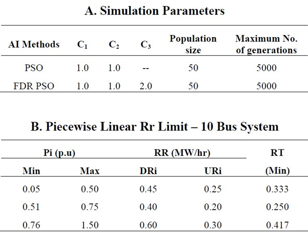
The optimal power dispatch and minimum production cost of the IPPs were obtained using swarm intelligence algorithms by satisfying the transient stability limits and transmission line constraints. The simulation parameters of the swarm intelligence methods which decide the execution time of the algorithms are given in Appendix A. A linearly decreasing inertia weight W, which varies from 0.9 to 0.2, was used for the convergence characteristics. The line flows were computed using Newton Raphson method and their thermal power limits were satisfied. The simulation studies were carried out on P IV, 3 GHz system in MATLAB environment. The effectiveness of the proposed method has been demonstrated by considering 10 bus and 26 bus test systems.
5.1 10 Bus System
The swarm intelligence algorithms were tested on ten bus system having 5 power producers and 13 transmission lines. The fuel cost coefficients, unit limits of the test system are taken from [24].
5.1.1 Case 1: Base Load Condition
The base load of the 10 bus system is 2.25 p.u. The optimal power flow solution with transient stability limits has been obtained using the FDR PSO algorithm. The optimal settings of the power producers and the obtained minimum fuel cost values are compared with other optimization methods which are given in Table 1.
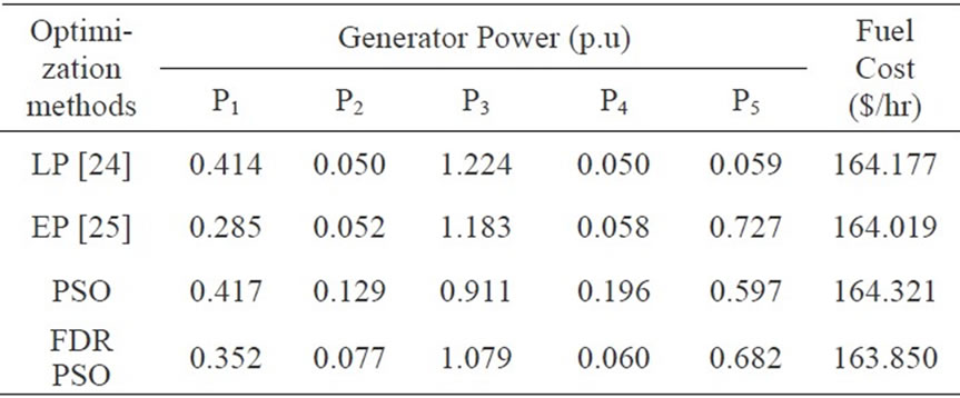
Table 1. Comparison among different methods
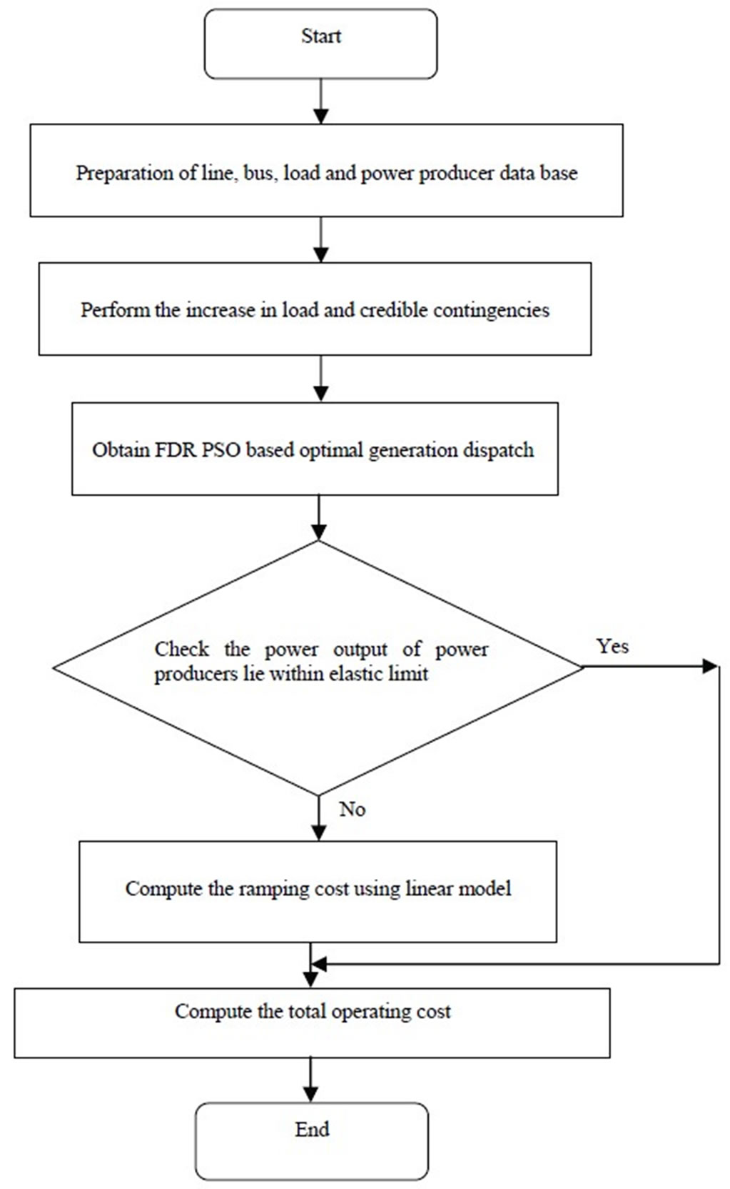
Figure 2. Step-by-step algorithm
From this table, it is inferred that the value of the fuel cost obtained through the proposed methods is better than the results obtained through other optimization methods. It was also observed that there was no vast variation in the five generator powers after several runs.
The convergence characteristics of PSO and FDR PSO methods are shown in Figure 3 for illustration. It is found that during initial iterations, FDR PSO concentrates mainly on finding feasible solutions to the problem. Then the value gradually settles down to the optimum value with most of the particles in the population reaching that point.
In the above OPF solution, the transient stability limit has to be incorporated by the following procedure: A three phase to ground fault was assumed in the transmission line connected between buses 8 and 9. The above fault was cleared by opening the contacts of the circuit breakers by 0.1 Section. The obtained OPF solution satisfies transient stability limits and the corresponding relative rotor angles of the generators are shown in Figure 4.
From this figure, it is observed that, while obtaining the solution for OPF problem, the relative rotor angles are also within safer limits and hence the system security is ensured.
5.1.2 Case 2: Production Cost with Ramping
The power producers have to change their generation
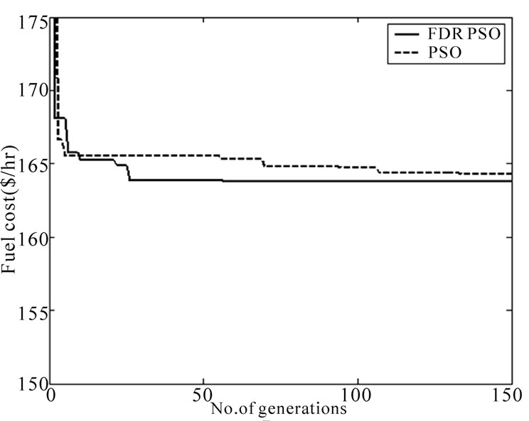
Figure 3. Convergence characteristics
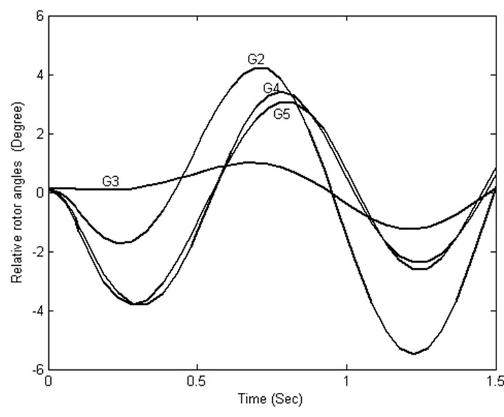
Figure 4. Relative rotor angle curves
schedule when the load changes. The operation of their settings depends upon their ramp rate limits. Initially, a stepwise ramping up/down limits is considered. The power producers are rescheduled to obtain their best setting point with various stepwise ramping limits. The obtained results are given in Table 2. From the table, it is inferred that the production cost is maximum when the producers operate with strict ramp rate limit and the minimum production cost is obtained when the ramp rate limit is around 20%. However, further stricter ramp rate constraint will restrict them from the essential diversity search, and result in more production cost or in less cost saving.
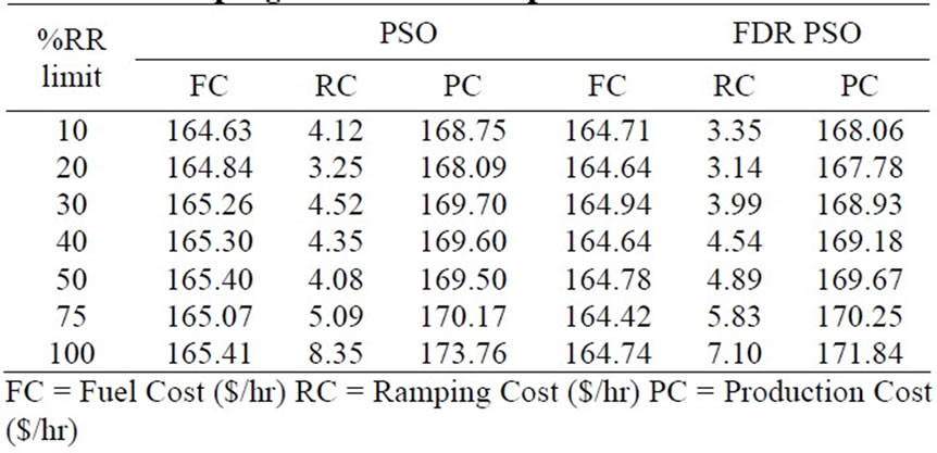
Table 2. Ramping cost results -stepwise RR limits
In reality, the power producers are operated with distinct ramping limits with respect to different operating conditions. Strict ramping limits increase the production cost while liberal ramping limits hurt the life of the rotor. Hence in this paper, a piecewise linear function is used to determine the ramping cost of the power producers. The piecewise linear ramp rate limits of the power producers are given in the Appendix B. The obtained optimal production cost of the power producers with piecewise linear ramping rate and transient stability limits using swarm intelligence methods is given in Table 3. Hence the proposed method is able to solve the real time ISO problem and able to handle non linear functions.
5.1.3 Case 3: Production Cost with Wheeling Transactions
In the restructured power market, most of the power transfers have been carried out through either bilateral or multilateral wheeling transactions. In this case, two simultaneous bilateral wheeling transactions and one multilateral transaction were carried out on the test system. The details of the wheeling transactions and magnitude of power transfer are given in Tables 4 and 5. PSO and FDR PSO methods are used to obtain the optimal production cost with linear ramp model for the practical power system and the results are given in Table 6. Whilesolving the above problem generator bus voltage limits, voltage angles, line flow limits and transformer tap positions are taken into account. The wheeling transactions are carried out in the system with transmission line MVA limits. Since the wheeling transactions are satisfying the transmission line limits, they are feasible.
5.2 26 Bus System
The swarm intelligence algorithms were used to obtain optimal production cost with linear ramp model for 26 bus utility system. It consists of six power producers and forty six transmission lines. The fuel cost coefficients, unit limits of the test system are taken from [26]. The piecewise linear ramp rate limits of the system are given Appendix C. The transient stability based OPF solution for the practical utility system was demonstrated with line and generator contingency case studies are illustrated in the following subsections.
5.2.1 Case 1: Optimal Production Cost with Line Contingency
In this case study, the optimal production solution of the test system is obtained through the FDR PSO algorithm when subjected to different types of line contingency (single line outage, during fault and double line outage) studies. 10% increase in base load condition is assumed. The transient stability limit of the power producers is also satisfied during the contingency based optimal solution procedure. The obtained OPF results for the various contingency case studies are consolidated in Table 7. It includes the minimum fuel and linear ramping costs incurred by the power producers and their corresponding settings. When the power limits of the power producers are violated during the contingency based rescheduling operation, then ramping cost is incurred, otherwise no ramping cost is levied. In Case (a), single line contingency is illustrated by making the line connected between buses 20 and 21 as out of service.
In Case (b), contingency based OPF solution is obtained
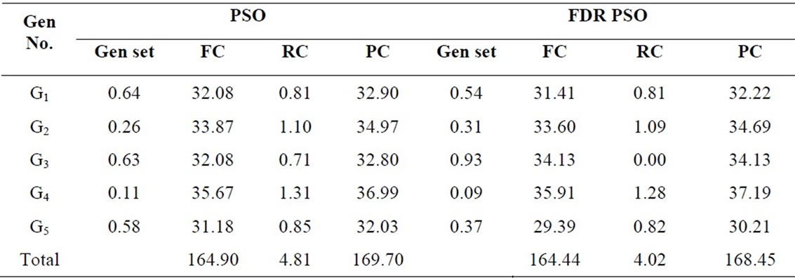
Table 3. Production cost -linear ramping
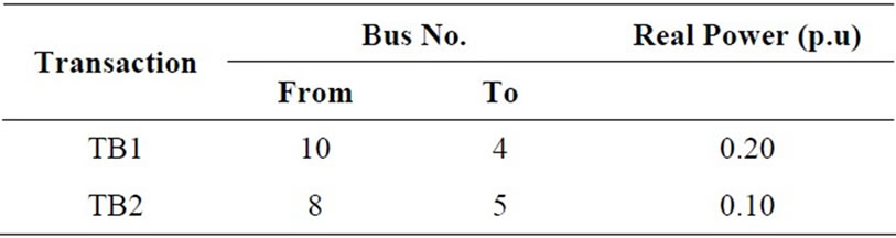
Table 4. Details of bilateral wheeling transactions
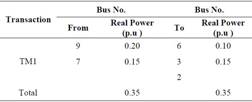
Table 5. Details of multilateral wheeling transactions
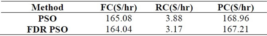
Table 6. Optimal production cost with wheeling transactions
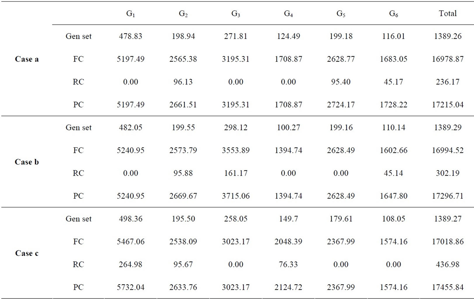
Table 7. OPF solution – line contingency case studies
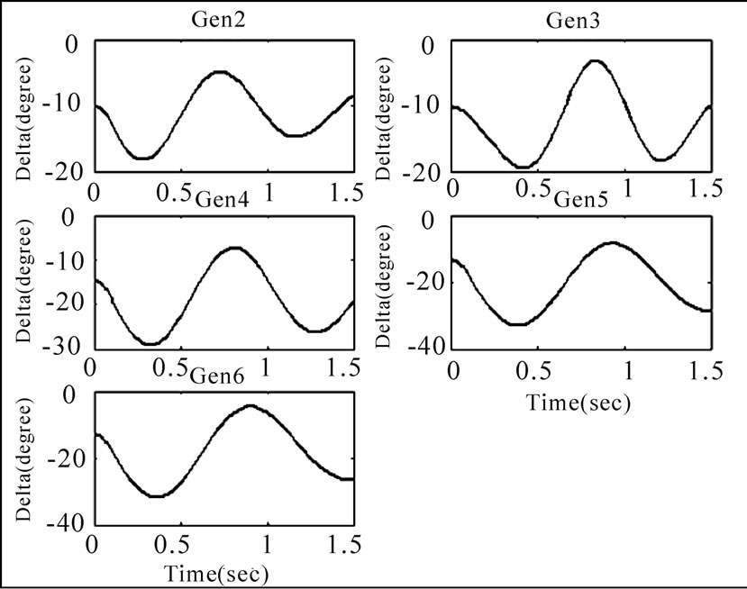
Figure 5. Relative rotor angles curve - Case b
Figure 6. Power Flow in transmission lines – Case c
during the fault condition. Along with the single line outage in the Case (a), a three phase to ground fault is also assumed in transmission line connected between buses 1 and 18. The fault is cleared by isolating the transmission line by 0.1 Sec. The corresponding relative rotor angle diagram with respect to the reference is given in Figure 5. It is inferred that the rotor angles of the power producers are within acceptable limits which ensures the system security.
In Case (c), two line contingencies are considered while obtaining the solution of the transient stability constrained OPF problem. The lines connected between buses (20-21) and (9-10) are made to be out of service to clear the fault. The power flow in the lines during the pre and post contingency conditions are shown in Figure 6. The obtained OPF solution satisfies the thermal power limits of the transmission lines during the credible contingencies.
5.2.2 Case 2: Generator Contingency Condition
A severe generator outage contingency based power flow solution is illustrated to demonstrate the effectiveness of the proposed FDR PSO approach. A generator connected at bus 5 is made out of service for maintenance purpose.
The minimum fuel, ramping and production costs for the above critical condition are obtained as 15604.31 $/hr, 639.16 $/hr 16243.47 $/hr respectively. The simulation results are shown in Figures 7 and 8 for rotor angles and angular frequencies respectively. From the waveforms shown in these figures, it can be concluded that the system remains stable since the waveforms do not diverge during the simulation interval.
6. Conclusions
FDR PSO algorithm for solving the OPF problem with credible contingencies considering transient stability constraints and piecewise linear ramping model are presented in this paper. The feasibility of the proposed
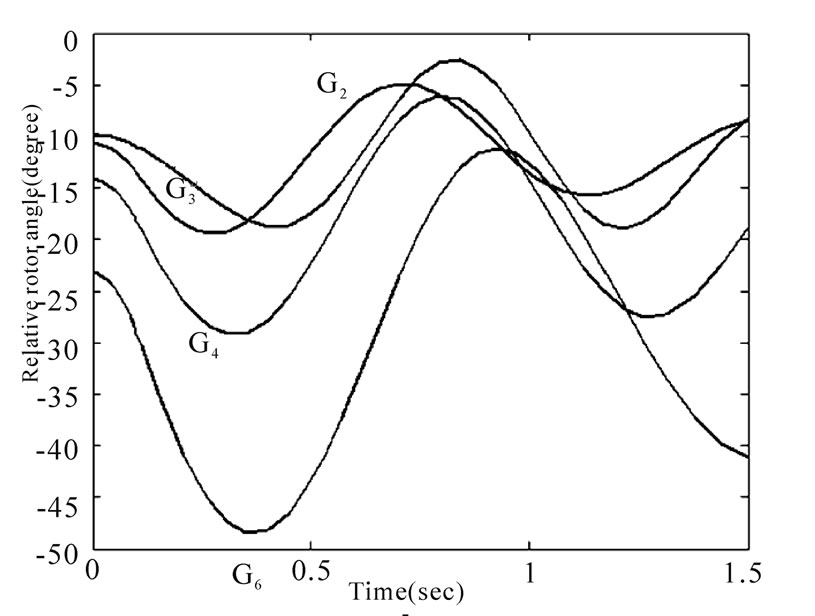
Figure 7. Relative rotor angle curves - Generator contingency condition
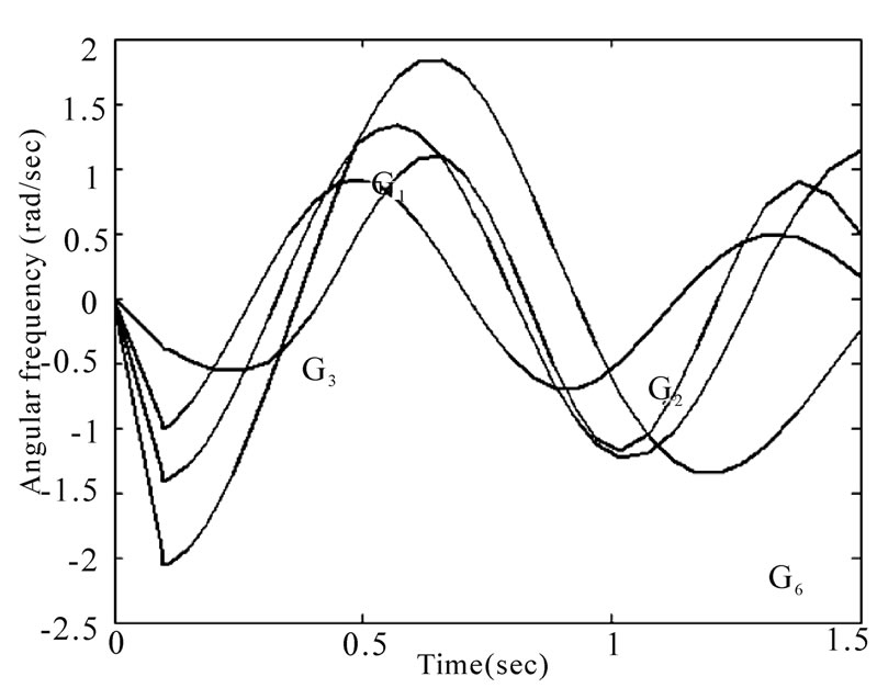
Figure 8. Angular frequency diagram - Generator contingency condition
method for solving the transient stability constrained OPF problem was demonstrated with two test systems considering various contingencies and nonlinearities like piecewise linear ramping model. The computation of linear ramping cost illustrates the increase in production cost of the power producers when subjected to load changes in the deregulated environment. The obtained results give feasible economic and security signals to the power utilities when subjected to vulnerable conditions in the deregulated power industry.
REFERENCES
- R. C. Bansal, “Optimization methods for electric power systems: An overview,” International Journal of Emerging Electric Power Systems, Vol. 2, No. 1, Article 1021, 2005.
- J. G. Vlachogiannis and K. Y. Lee, “A comparative study on particle swarm optimization for optimal steady-state performance of power systems,” IEEE Transactions on Power Systems, Vol. 21, No. 4, pp. 1718–1728, November 2006.
- I. Selvakumar and K. Thanushkodi, “A new particle swarm optimization solution to non convex economic dispatch problems,” IEEE Transactions on Power Systems, Vol. 22, No. 1, pp. 42–51, February 2007.
- P. E. Onate Yumbla, J. M. Ramirez, and C. A. Coello, “Optimal power flow subject to security constraints solved with a Particle swarm optimizer,” IEEE Transactions on Power Systems, Vol. 23, No. 1, pp. 33–40, February 2008,.
- M. Ni, J. D. McCalley, V. Vittal, T. Tayyib, “Online Risk-based security assessment,” IEEE Transactions on Power Systems, Vol. 18, No. 1, pp. 258–265, February 2003.
- US-Canada Power System Outage Task Force, Final Report on the August 14, 2003 Blackout in the United States and Canada: Causes and Recommendations, Issued April 2004.
- D. Gan, R. J. Thomas, R. D. Zimmerman, “Stability constrained optimal power flow,” IEEE Transactions on Power Systems, Vol. 15, No. 2, pp.535–540, 2000.
- D.-H. Kuo and A. Bose, “A generation rescheduling method to increase the dynamic security of power systems,” IEEE Transactions on Power Systems, Vol. 10, No. 1, pp. 68–76, February 1995.
- N. Mo, Z. Y. Zou, K. W. Pong, and T. Y. G. Pong, “Transient stability constrained optimal power flow using particle swarm optimization”, IET. Generation, Transmission and Distribution, Vol. 1, No. 3, pp. 476–483, 2007.
- X. J. Lin, C. W. Yu, and A. K. David, “Optimum transient security constrained dispatch in competitive deregulated power systems,” Electric Power Systems Research, Vol. 76, pp. 209–216, 2006.
- W. Gu, F. Milano, P. Jiang, and J. Y. Zheng, “Improving large-disturbance stability through optimal bifurcation control and time domain simulations,” Electric Power Systems Research, Vol. 78, pp. 337–345, 2008.
- S. V. Ravikumar and S. S. Nagaraju, “Transient stability improvement using UPFC and SVC,” ARPN Journal of Engineering and Applied Sciences, Vol. 2, No. 3, pp. 38–45, June 2007.
- C. Wang and S. M. Shahidehpour, “Optimal generation scheduling with ramping costs,” IEEE Transactions on Power Systems, Vol. 10, No. 1, pp. 60–67, February 1995.
- G. B. Shreshtha, K. Song, and L. Goel, “Strategic selfdispatch considering ramping costs in deregulated power markets,” IEEE Transactions on Power Systems, Vol. 19, No. 3, pp. 1575–1581, August 2004.
- M. Tanaka, “Real time pricing with ramping costs: A new approach to managing a steep change in electricity demand,” International Journal of Energy Policy, Vol. 34, No. 18, pp. 3634–3643, December 2006.
- F. Li and R. M. D. Williams, “Towards more cost saving under stricter ramping rate constraints of dynamic economic dispatch problems—A genetic based approach,” Proceedings of the IEEE International Conference on Genetic algorithms in Engineering Systems: Innovations and Applications, 2–4 September 1997.
- California Independent System Operator, United States of America (www.caiso.com).
- Midwest Independent System Operator, United States of America (www.midwestiso.org).
- T. Li and M. Shahidehpour, “Dynamic ramping in unit commitment,” IEEE Transactions on Power Systems, Vol. 22, No. 3, pp. 1379–1381, August 2007.
- J. Kennedy and R. Eberhart, “Particle swarm optimization,” Proceedings of the IEEE International Conference on Neural Networks, Vol. 4, pp. 1942–1948, December 1995.
- E. Ozcan and C. K. Mohan, “Particle swarm optimization: surfing the waves,” Proceedings of the Congress on Evolutionary Computation (CEC’99), Washington D.C., pp. 1939–1944, July 1999.
- M. Clerc and J.Kennedy, “The particle swarm: Explosion, stability and convergence in a multi-dimensional complex space,” IEEE Transactions on Evolutionary Computation, Vol. 6, pp. 58–73, 2002.
- T. Peram, K. Veeramacheneni, and C. K. Mohan, “Fitness distance ratio based particle swarm optimization,” Proceedings of the IEEE Swarm intelligence Symposium, 24–26, pp. 174–181, April 2003.
- A. Farag, S. Al-Baiyat, and T. C. Cheng, “Economic load dispatch multiobjective optimization procedures using linear programming techniques,” IEEE Transactions on Power Systems, Vol. 10, No. 2, pp. 731–737, May 1995.
- R. Gnanadass, K. Manivannan, and T. G. Palanivelu, “Application of evolutionary programming approach to economic load dispatch problem,” National Power System Conference, IIT, Kharagpur, 2002.
- H. Saadat, “Power system analysis,” McGraw-Hill Publication, Chapter 7, pp. 300–302, 1999.
Appendix