Int'l J. of Communications, Network and System Sciences
Vol.3 No.1(2010), Article ID:1179,4 pages DOI:10.4236/ijcns.2010.31012
Novel Approach to Improve QoS of a Multiple Server Queue
1Reliance Technology Innovation Center, Reliance Communication, Mumbai, India
2Department of Electronics,Lokmanya Tilak College of Engg, Mumbai, India
3Department of E & TC, Dr. Babasaheb Ambedkar Technological University, Lonere, Raigad, India
E-mail: {munir.sayyad, ktsmanian}@gmail.com, {powerabhik, nalbalwar_sanjayan}@yahoo.com
Received October 24, 2009; revised November 26, 2009; accepted December 27, 2009
Keywords: QoS, SIP, S S Queue, M S Queue
Abstract
The existing models of servers work on the M/G/1 model which is in some ways predictable and offers us an opportunity to compare the various other server queuing models. Mathematical analysis on the M/G/1 model is available in detail. This paper presents some mathematical analysis which aims at reducing the mean service time of a multiple server model. The distribution of the Mean Service Time has been derived using Little’s Law and a C++ simulation code has been provided to enable a test run so that the QoS of a multi-server system can be improved by reducing the Mean Service Time.
1. Introduction
In queuing theory, a queuing model is used to approximate a real queuing situation or system, so the queuing behavior can be analyzed mathematically. Queuing models allow a number of useful steady state performance measures to be determined, including:
• The average number in the queue, or the system
• The average time spent in the queue, or the system
• The statistical distribution of those numbers or times
• The probability the queue is full, or empty, and The probability of finding the system in a particular state.
Queuing models are often set up to represent the steady state of a queuing system, that is, the typical long run or average state of a system. As a result, these are stochastic models that actually represent and symbolize the probability that a queuing system will be found in a particular configuration or state [1].
2. Single Server Queue
Single-server queues are, perhaps, the most commonly encountered queuing situation in real life. One encounters a queue with a single server in many situations, including business (e.g. sales clerk), industry (e.g. a production line), transport (e.g. a bus, a taxi rank, an intersection), telecommunications (e.g. Telephone line), computing (e.g. processor sharing). Even where there are multiple servers handling the situation it is possible to consider each server individually as part of the larger system, in many cases. (E.g. A supermarket checkout has several single server queues that the customer can select from.) Consequently, being able to model and analyze a single server queue’s behavior is a particularly useful thing to do.
2.1. Poisson Arrivals and Service
M/M/1/∞/∞ represents a single server that has unlimited queue capacity and infinite calling population, both arrivals and service are Poisson (or random) processes, meaning the statistical distribution of both the inter-arrival times and the service times follow the exponential distribution [3].
2.2. Poisson Arrivals and General Service
M/G/1/∞/∞ represents a single server that has unlimited queue capacity and infinite calling population, while the arrival is still Poisson process, meaning the statistical distribution of the inter-arrival times still follow the exponential distribution, the distribution of the service time does not.
2.3. Infinitely Many Servers
While never exactly encountered in reality, an infinite-servers (e.g. M/M/∞) model is a convenient theo-

Figure 1. Components of a basic queuing process.
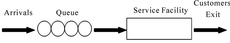
Figure 2. Single server queue.
retical model for situations that involve storage or delay, such as parking lots, warehouses and even atomic transitions. In these models there is no queue, as such; instead each arriving customer receives service. When viewed from the outside, the model appears to delay or store each customer for some time.
3. Multiple Server Queue
Multiple (identical)-Server Queue situations are frequently encountered in telecommunications or a customer service environment. When modeling these situations care is needed to ensure that it is a multiple servers queue, not a network of single server queues, because results may differ depending on how the queuing model behaves.
One observational insight provided by comparing queuing models is that a single queue with multiple servers performs better than each server having their own queue and that a single large pool of servers performs better than two or more smaller pools, even though there are the same total number of servers in the system [4,5].
Queuing models can be represented using Kendall's notation:
A/B/S/K/N/Disc where:
• A is the inter arrival time distribution
• B is the service time distribution
• S is the number of servers
• K is the system capacity
• N is the calling population
• Disc is the service discipline assumed Many times the last members are omitted, so the notation becomes A/B/S and it is assumed that K = ∞, N = ∞and Disc = FIFO.
Some standard notations for distributions (A or B) are:
• M for Markovian (exponential) distribution
• Eκ for an Erlang distribution with κ phases
• D for Degenerate (or Deterministic) distribution (constant)
• G for General distribution (arbitrary)
• PH for a Phase-type distribution The basic notations in the queuing model that we are about to mathematically analyze are:
Λ = Arrival rate E (B) = Mean Service Time Amount of work per unit time = λ E(B)
For a multiple server, p is the occupation rate or server utilization.
p = [λ E(B)] / c Here c is the number of servers.
Therefore, p α 1 / c Thus, the more number of servers, the lesser will be the occupation rate i.e. server utilization [7,8].
One simple example : Consider a system having 8 input lines, single queue and 8 servers. The output line has a capacity of 64 Kbit/s. If we assume the arrival rate at each input to be 2 packets/s, then, the total arrival rate is 16 packets/s. With an average of 2000 bits per packet, the service rate is 64 Kbit/s/2000b = 32 packets/s. Hence, the average response time of the system is 1/(μ − λ) = 1/(32 − 16) = 0.0625 sec. Now, consider a second system with 8 queues, one for each server. Each of the 8 output lines has a capacity of 8 Kbit/s. The calculation yields the response time as 1/(μ − λ) = 1/(4 − 2) = 0.5 sec. And the average waiting time in the queue in the first case is ρ/(1 − ρ)μ = 0.03125, while in the second case is 0.2.
4. Little’s Law
In queuing theory, Little's result, theorem, lemma, or law says: The long-term average number of customers in a stable system L (known as the offered load), is equal to the long-term average arrival rate, λ, multiplied by the long-term average time a customer spends in the system, W, or :
L = lW Although it looks intuitively reasonable, it's a quite remarkable result, as it implies that this behavior is entirely independent of any of the detailed probability distributions involved, and hence requires no assumptions about the schedule according to which customers arrive or are serviced. Imagine a small shop with a single counter and an area for browsing, where only one person can be at the counter at a time, and no one leaves without buying something. So the system is roughly:
Entrance → Browsing → Counter → Exit This is a stable system, so the rate at which people enter the store is the rate at which they arrive at the counter and the rate at which they exit as well. We call this the arrival rate.
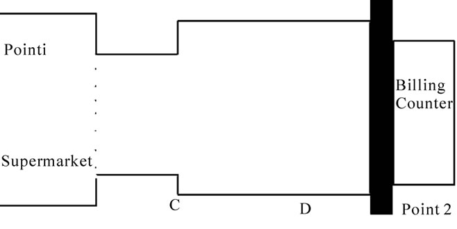
Figure 3. Little’s law represemtation.
Little's Law tells us that the average number of customers in the store, L, is the arrival rate, λ, times the average time that a customer spends in the store, W, or simply :
L = lW
5. Usage of Little’s Law for MSMA
We can also say that E(L) = λE(S).
From Figure 3 we can say that.
Mean number of customers in ABCD = Avg. number of customers x Mean sojourn time Replacing the parameters with standardized server parameters:
E(L) will be the occupation rate
Λ will be arrival rate i.e. average rate of packets arriving per unit time.
E(S) will be mean service time.
Now, based on theory of probability distribution E(X) = ∑ pixi
Let us assume the following model:
Let X represent the number of packets occupying the server.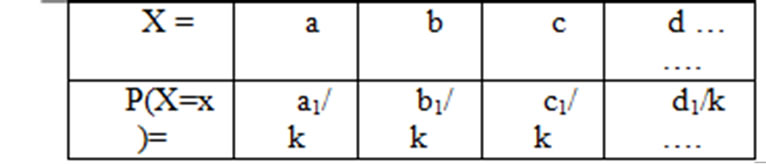
where k is the ideal occupation time and a1, b1, c1, d1 are the actual occupation times.
NowE(X) = ∑ pixi
= a1/k (a) + b1/k (b) + c1/k (c) + d1/k (d) + …..
=1/k [a1(a) + b1(b) + c1(c) + d1(d) + …… ]
Therefore, condition for mapping will be:
1/k [a1(a) + b1(b) + c1(c) + d1(d) + …… ] <= E(L)
where E(L) is the mean occupation rate.
SinceE(L) = λ E(S)
1/k [a1(a) + b1(b) + c1(c) + d1(d) + …… ] <= λ E(S)
(1/k [a1(a) + b1(b) + c1(c) + d1(d) + …… ]) / λ = E(S)
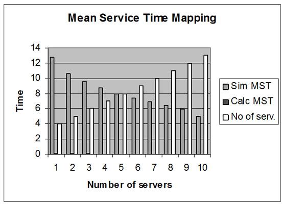
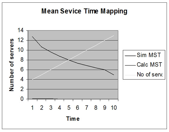
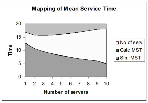
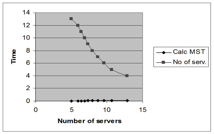
Therefore, the basic aim of this mathematical analysis is provide a standard relation so that a distribution graph can be plotted against the graph for E(S) (Mean Service Time) to make them as similar as possible.
6. Conclusions
In a multiple server system, based on the derived mathematical model, a simulation can be carried out using the provided C++ simulator. The following conclusions can be drawn from the test:
The arrival rate increases as we increase the number of servers owing to the increase in the number of input lines. The occupation rate decreases as there are more number of servers to handle the load. The Mean Service Time will therefore decrease as we increase the number of servers, thus there will be more firepower to handle the packet load. The processing will be shared among the different servers. This will help in improving the QoS. The simulation software will provide us with a chance to test random data values and validate the theory.
7. Results
8. References
[1] C. M. Grinstead and J. L. Snell, “Introduction to probability,” American Mathematical Society.
[2] G. Giambene, “Queuing theory and telecommunications : Network and applications.”
[3] K. H. Kumar and S. Majhi, “Queuing theory based open loop control of Web server,” IEEE Paper, 2004.
[4] J. P. Lehoczky, “Using real-time queuing theory to control lateness in real-time systems,” 1997.
[5] F. Spies, “Modeling of optimal load balancing strategy using queuing theory,” 2003.
[6] J. S. Wu and P. Y. Wang, “The performance analysis of sipt signaling system in carrier class VOIP network,” IEEE Paper, 2003.
[7] C. M. Grinstead and J. L. Snell, “Introduction to probability,” American Mathematical Society.
[8] M. Veeraraghavan, “Derivation of little’s law,”.