Journal of Water Resource and Protection
Vol.6 No.4(2014), Article ID:44283,14 pages DOI:10.4236/jwarp.2014.64036
Characterization of Groundwater Pollution Sources with Unknown Release Time History
Om Prakash1,2*, Bithin Datta1,2
1Discipline of Civil and Environmental Engineering, School of Engineering and Physical Sciences, James Cook University, Townsville, Australia
2CRC for Contamination Assessment and Remediation of the Environment, Mawson Lakes, Australia
Email: *om.prakash@my.jcu.edu.au, bithin.datta@jcu.edu.au
Copyright © 2014 by authors and Scientific Research Publishing Inc.
This work is licensed under the Creative Commons Attribution International License (CC BY).
http://creativecommons.org/licenses/by/4.0/


Received 27 November 2013; revised 26 December 2013; accepted 23 January 2014
ABSTRACT
Characterizations of unknown groundwater pollution sources in terms of source location, source flux release history and sources activity initiation times, from sparse observation concentration measurements are a challenging task. Optimization-based methods are often applied to solve groundwater pollution source characterization problem. These methods are effective only when the starting times of activity of the sources are precisely known, or the possible time window within which the sources activity actually start is known with a fair degree of certainty. However, in real life scenarios, the starting time of the activity of the sources is either unknown or can lie anywhere within a time window of years or decades. Absence of any prior information about the span of time window, within which the sources become active, makes existing source identification methodologies inefficient. As an alternative, an optimization-based source identification model is proposed, to simultaneously estimate source flux release history and sources activity initiation times. The method considers source flux release history and sources activity initiation times as explicit decision variables, optimally estimated by the decision model. Performance of the developed methodology is evaluated for an illustrative study area having multiple sources with different source activity initiation times, missing observation data and transient flow conditions. These evaluation results demonstrate the potential applicability of the proposed methodology and its capability to correctly estimate the unknown source flux releasing history and sources activity initiation times.
Keywords: Groundwater Pollution; Pollution Source Identification; Unknown Pollution Source Starting Time; Linked Simulation Optimization; Simulated Annealing

1. Introduction
In the event of detection of any pollutant in the groundwater system, the next step is to design an effective remediation strategy for reclaiming a polluted aquifer. This requires precise information of the source characteristics in terms of source location, source flux release history and sources activity initiation times. The process of flow and transport in the groundwater system is so slow, that many times pollution in an aquifer is detected much after the pollution sources have become active or may even have ceased to exist. Therefore, even a rough guess of the time span within which the source activity has started may be very difficult.
Optimization based methodologies developed so far for unknown source flux characterization which relies on some knowledge of the approximate starting time of the sources activities. In all real world problems, the starting time of the activity of the sources is either unknown or can lie anywhere within a time window of years or decades. Absence of any prior information about the starting time of activity of the pollution sources, or the span of time window, within which the sources becomes active, renders the existing source identification methodologies inefficient. To overcome this, a methodology is developed for simultaneously estimating source flux releasing history and sources activity initiation times, using a new optimal decision model that can efficiently solve the source characterization problem, when it is impossible to specify a small time span within which the source activity may have started.
Unknown groundwater pollution sources characterization is non-linear [1] , ill-posed inverse problem [2] . Initial contributions in identification of unknown groundwater pollution sources proposed the use of linear optimazation model based on linear response matrix approach [3] and the use of statistical pattern recognition [4] . Some of the important contributions to solve the problem of identifying unknown groundwater pollution sources include reverse time random particle method for finding the most probable source [5] ; non-linear maximum likelihood estimation based inverse models to determine optimal estimates of the unknown model parameters and source characteristics [6] ; minimum relative entropy, a gradient based optimization for solving source identification problems [7] [8] [9] ; embedded nonlinear optimization technique for source identification [10] [11] ; inverse procedures based on correlation coefficient optimization [12] ; Tikhonov regularization [13] [14] ; quasireversibility [15] [16] ; marching-jury backward beam equation [17] [18] ; genetic algorithm based approach [19] , [20] [21] ; artificial neural network approach [22] [23] [24] ; classical optimization based approach [25] [26] [27] ; Probabilistic Support Vector Machines (PSVMs) and Probabilistic Neural Networks (PNNs) based probabilistic models [28] ; inverse particle tracking approach [29] [30] ; heuristic harmony search for source identification [31] ; Simulated Annealing (SA) as optimization for source identification [32] [33] . A review of different optimization techniques for solving source identification is presented in [34] and [35] . An extensive overview of various stochastic and deterministic approaches for solving groundwater pollution problem can be found in [36] and [37] .
All existing optimization based source identification techniques implicitly assume that the starting time of the activity of the sources is precisely known, or the time span for the possible start of the sources activity is known with fair degree of certainty. This is because, in the existing methodologies, the starting time is not treated as an explicit decision variable, but generally estimated indirectly by solving for source fluxes magnitudes at defined discretised time intervals. The following scenarios represent the existing methods and their limitations.
1) The actual starting time of the source activity is assumed to be precisely known. This is an impractical assumption and in all real world scenarios, there is seldom any clue about the actual starting time of the sources. As a result most of these developed methods cannot be applied to such real world scenarios.
2) In scenarios where the time span for the possible start of the sources activities is known with fair degree of certainty, a typical range being of 1 to 5 years, the precise actual starting time of the sources is estimated indirectly by estimating the source fluxes magnitude for entire time span, discretised into smaller stress periods. As a result, large number of decision variables is added to the optimization problem. Each of these decision variables represent the source flux magnitude for a potential/actual source for a given stress period. Hence, the optimization problem needs to be solved for a large number of source flux magnitudes at different time intervals. Such a solution may theoretically seem possible but with every added decision variable, the dimension of the search space increases, leading to exponential rise in the computational time. This indirect approach does not represent an efficient formulation of the optimum decision model.
3) In the third scenario where there is no information of time span for the possible start of the sources activities, solution of source identification becomes highly challenging. If the solution approach as discussed for the previous scenario is applied to solve for the actual starting time, would mean solving for hundreds of source flux magnitudes for a very large number of stress periods, for a very large time span. This would not only increase the size of the optimization problem, but may render it computationally infeasible.
4) The solution methodology for all the above mentioned scenarios implicitly assumes that the actual starting time of the sources will always lie within a specified time span considered in the study. If this is untrue, the existing methods fail to give any meaningful result.
To address these limitations, a new methodology is proposed for simultaneously identifying the starting times of the activity of the sources and their flux release history. A new optimum decision model is formulated and solved for this purpose. SA is used for solving the optimization problem with starting times of the sources as the explicit decision variable. Performance of the proposed methodology is evaluated by solving an illustrative example problem for different sources activity initiation time scenarios, transient flow conditions and missing observation data to demonstrate its potential applicability.
2. Methodology
The proposed methodology incorporates the starting time of the activity of the source as explicit unknown variable in the optimization based decision model. Simulated Annealing is used for solving the optimization problem with an objective of minimizing the residual error between the simulated and observed pollutant concentrations measurements at observed locations. The optimization model is solved such that the unknown source fluxes and the stating times of the activity of the sources are the direct solutions of the source identification problem.
2.1. Source Identification Using Linked Simulation-Optimization Model
A linked simulation optimization model simulates the physical process within the optimization model. Therefore the simulation model is treated as a set of binding constraints for the optimization model. Therefore any feasible solution of the optimization model needs to satisfy the flow and the transport simulation model. The advantage of this approach is that it is possible to link any complex numerical model to the optimization model. In this simultaneous optimal source flux and activity starting time identification model, the flow and transport simulation models are linked to the optimization model using the SA algorithm for solution.
2.2. Groundwater Flow Simulation Model
A three dimensional numerical model MODFLOW [38] is used to simulate the groundwater flow in the polluted aquifer. MODFLOW is a computer program that numerically solves the three-dimensional groundwater flow equation for a porous medium by using a finite-difference method. The partial differential equation for groundwater flow [39] is given by equation (1):
 (1)
(1)
where Kxx, Kyy and Kzz represent the values of hydraulic conductivity along the x, y and z coordinate axes (LT−1)
h is the potentiometric head (L)
W is the volumetric flux per unit volume representing sources and/or sinks (T−1)
Ss is the specific storage of the porous material (L−1)
t is time (T)
x, y and z are the cartesian co-ordinates (L)
2.3. Solute Transport Model in Groundwater System
A three dimensional modular pollutant transport model MT3DMS [40] is used to simulate the solute transport in the polluted aquifer system. The transport model (MT3DMS) utilizes the flow field generated by the flow model (MODFLOW) to compute the pollutant plume. The partial differential equation describing three-dimensional transport of pollutants in groundwater [41] is given by equation (2).
 (2)
(2)
where C is the concentration of pollutants dissolved in groundwater (ML−3)
t is time (T)
xi is the distance along the respective Cartesian coordinate axis (L)
Dij is the hydrodynamic dispersion coefficient tensor (L2T−1)
vi is the seepage or linear pore water velocity (LT−1); it it is related to the specific discharge or Darcy flux through the relationship, vi = qi/θ
qs is volumetric flux of water per unit volume of aquifer representing fluid sources (positive) and sinks (negative) (T−1)
Cs is the concentration of the sources or sinks (ML−3)
θ is the porosity of the porous medium (dimension less)
 is chemical reaction term for each of the N species considered (ML−3T−1).
2.4. Optimization Model
Simulated Annealing (SA) is used as an optimization algorithm to solve the optimization problem. Simulated Annealing was first introduced by [42] , is an extension of the metropolis algorithm [43] . The basic concept of SA is derived from thermodynamics. Each step of SA algorithm replaces the current solution by a random nearby solution, chosen with a probability that depends on the difference between the corresponding function values and algorithm control parameters (initial temperature, temperature reduction factor etc.).
2.5. Simultaneous Source Flux and Activity Starting Time Identification Model
In source identification problem where the starting times of the activity of the sources is known, temporal pollutant source fluxes from all the potential sources, represented by the term  in the transport Equation (2) are the only explicit decision variable. Source flux identification using linked simulation-optimization is solved by minimizing the difference between the simulated and the observed concentration measurements in space and time. Hence, source identification problems need observed concentration measurement data at different locations and times. Actually, typical concentration measurements at a given observation location, represents only a small portion of the entire concentration versus time plot (breakthrough curve) measured at discrete time intervals, as shown in figure 1. If multiple sources are active at different locations and times, the concentration measurements at an observation location over a period of time represent a portion of the combined breakthrough curve at that observation location.
If the starting time of the activity of the sources is assumed to be known, the simulated concentration measurements can be correctly mapped in time to the observed concentration measurements to calculate the residual error at the observed locations. However, in real life scenario, the starting time of the source is mostly unknown. Hence it becomes unclear which temporal concentration measurement values on the simulated breakthrough curve, corresponds in time to the observed concentration measurements, and can be used to calculate the residual error at the observed locations. This can be understood from the illustrative example shown below.
Figure 2 shows pollutant plumes in the polluted aquifer at 1200, 1400, 1600 and 1800 days since the start of any source activity. It is evident from figure 2, that the pollutant plume is dynamic in nature. This implies that the observed concentration measurement at an observation location will vary in magnitude when taken at different times. However, if the starting time of the sources is unknown, it cannot be determined if the resulting plumes and the corresponding concentration measurements are for 1200, 1400, 1600 and 1800 days since the start of any source activity, or for a different set of days. A meaningful comparison between the observed pollutant plumes and the simulated pollutant plumes is only possible when they correspond to the same time. Hence a correct estimate of the source fluxes is only possible when the actual and estimated plumes are compared co-
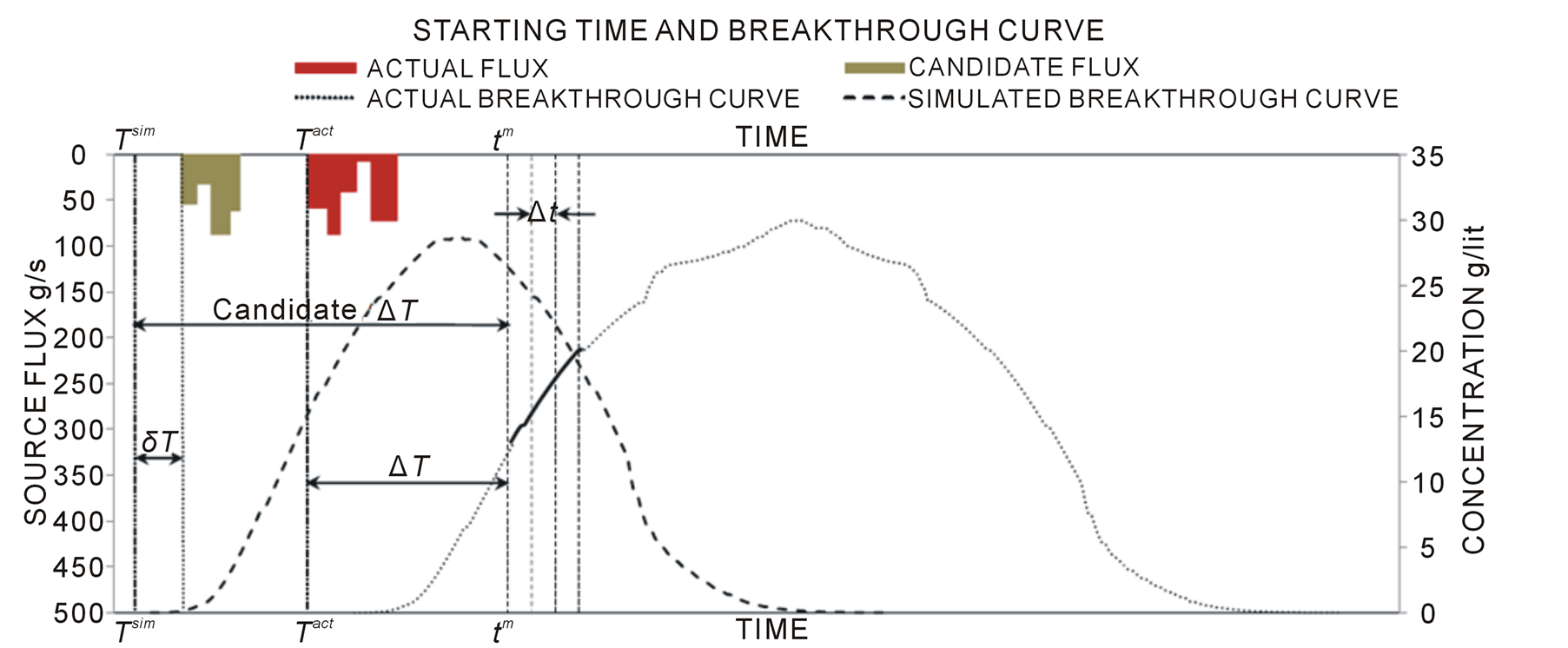
Figure 1.Details of variables with respect to an observed breakthrough curve at a monitoring location.
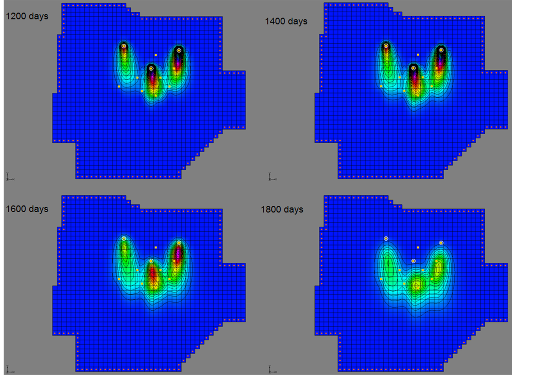
Figure 2.Pollutant plume in the polluted aquifer study area at different times.
rrectly in time and space. Hence, the time lags between the start of the activity of the sources and the observed concentration measurement needs to be ascertained in order to estimate the sources activity starting times.
To overcome the limitation of the earlier proposed methodologies, an explicit decision variable, time lag  as explained below is defined in the source identification model.
  is the time between the first concentration measurement and the actual source activity initiation time. Figure 1 shows a typical breakthrough curve at any observation location
  with the source activity plotted on the x axis. The x axis represents the time axis, primary y axis represents the source flux (g/s) and the secondary y axis represents the concentration of the dissolved pollutant in groundwater at observation location
  (g/lit). Only a small portion of the breakthrough curve, shown by solid line in figure 1, represents concentration measurements of the pollutant at observation location
 .
.
The following variables are used in the formulation of the source identification model:
 = a calendar date representing the actual starting time of the activity of a source;
 = a calendar date representing the starting time of the simulation for any particular candidate solution in the optimization model;
 = time interval between the starting time of the simulation and the starting time of the activity of source
 , for any particular candidate solution in the optimization model (i is an integer variable varying from 1to maximum number of sources);
 = a calendar date representing the first concentration measurement obtained from the site;
 = time interval between concentration measurements; (T)
N = number of concentration measurements available (assumed same for all measurement locations) such that

 = observed concentration measurement at observation location
  at time
  (ML−3);
 = corresponding simulated concentration at observation location
  at time
  (ML−3).
The objective function is defined as:
 (3)
(3)
 (4)
(4)
 (5)
(5)
Subject to
 (6)
(6)
where  represents the simulated concentration obtained from the transport simulation model at an observation location at time t and source flux
 :
:
 is the total number of concentration measurement wells;
 is the absolute difference.
The constraint set in equation (6) essentially represents the linking of the optimization algorithm with the numerical groundwater flow and transport simulation model through the decision variables. The optimization algorithm searches for optimal values of unknown pollutant source fluxes,  the lag time
  and
and 
(i is an integer variable varying from 1 to maximum number of sources) by generating candidate solutions of these decision variables in optimization algorithm. Candidate values of fluxes  are used as input for simulations of flow and transport models. Thus the lag time between the start of any source
  and first concentration measurement obtained from the site is given by
 .
.
This optimal search process with different candidate values of unknown variables results in an optimal solution that minimizes residual error between the simulated and observed pollutant concentrations. It is to be noted that  and
and  are decision variables whose value is to be optimally determined to ascertain the times of initiation of the pollutant source fluxes. The optimal value of lag time
  and
and  gives the best estimate of the actual source fluxes starting times
  obtained as solution.
3. Performance Evaluation of Developed Methodology
The performance of the proposed methodology is evaluated for an illustrative polluted aquifer study area as shown in figure 3. The performance is evaluated for different scenarios by varying source activity initiation times, varying the degree of spatial heterogeneity in the study area and different combination of observation locations. The study area is specified as comprising of heterogeneous, anisotropic, and confined aquifer. This study area has total dimension of 2100 meters in the x direction and 1950 meters in the y direction. The entire study area is discretised into smaller grids of size Δx, Δy and Δz in x, y and z direction respectively. The study area contains three different hydro-geological zones with different values of hydraulic conductivity Kxx and po-
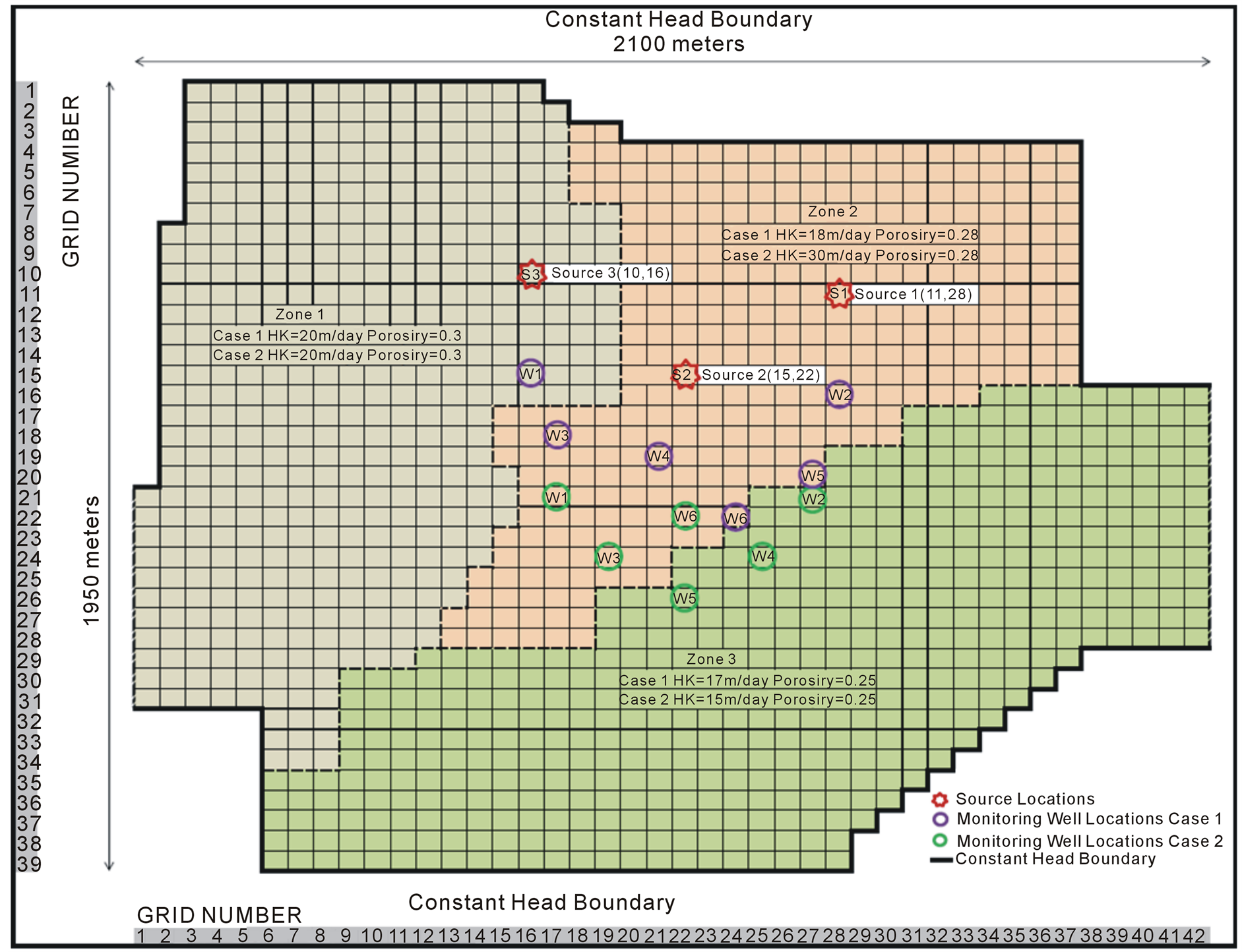
Figure 3. Plan view of the illustrative study area.
rosity θ. Groundwater flow and solute transport processes are simulated using the value for saturated thickness of the aquifer b, longitudinal dispersivity αL, transverse dispersivity αT and horizontal anisotropyas given in table 1.
In the discretised study area, cells marked with red star represent the grid locations containing a pollutant source S(i) where i represents the source number. Cells marked with green and purple circles are the grid locations containing an observation well.
In the first scenario, all the three sources are assumed to have different activity initiation times (table 2) and activity duration of 900 days. The entire activity duration of the sources is divided into three equal stress periods of 300 days. The pollutant flux from the sources is assumed to be constant over a stress period. The pollutant flux from each of the sources is represented as S(i)(j), where i represents the source number and j represents the stress period number. A total of nine source fluxes S11, S12, S13, S21, S22, S23, S31, S32, S33,  ,
, ,
, and
and  are considered as explicit unknown variables in the optimization problem. The hydraulic conductivity Kxx and effective porosity θ values in the three zones are kept different to show heterogeneity in the aquifer system. The scenario is further complicated by considering irregular monitoring for pollutant concentration measurements and missing observation measurement data Cobs.
Since all flow and pollutant transport in groundwater system is inherently transient, the performance of the developed methodology was evaluated for transient flow and solute transport condition in the second scenario. Three different sources are considered and it is assumed that all the three sources start activity at the same time. It is also assumed that the starting time of the activity of the sources is same as the starting time of the simulation , hence
 . The activity duration of the sources is divided into three equal stress periods of 364 days in this scenario. The pollutant flux from the sources is assumed to be constant over a

Table 1. Hydro-geological parameters for study area.
Table 2. Test case scenarios.
stress period. A total of nine source fluxes S11, S12, S13, S21, S22, S23, S31, S32, S33 and ∆T are considered as explicit unknown variables in the optimization problem.
4. Simulation of Observed Concentration
In actual field application, the concentration measurements are to be obtained from field data. However, for performance evaluation purpose, these measurements are synthetically generated by simulation for assumed actual pollutant sources. The observed aquifer responses are simulated by numerical simulation models, MODFLOW and MT3DMS in GMS7.0. Initial and boundary conditions i.e. initial heads, boundary heads are specified in the numerical simulation models. Actual source fluxes are utilized to simulate these observed concentration measurement data at specified measurement locations.
The time of start of the numerical simulation model for synthetically generating the observed concentration measurements is designated as the initial time . This initial time can be defined with respect to a calendar date, which in practice would correspond to the actual starting time of the sources. The time lag between the start of the numerical simulation model for synthetically generating the observed concentration measurements, and the first concentration measurement used for source identification is also specified.
In the first evaluation scenario considered, the time lag between the time of first pollutant concentration measurement  used in the source identification model, and the actual starting time of the sources activity
 , is 500, 200 and 800 days for source S1, S2 and S3, respectively. Concentration measurements are taken at discrete time intervals starting from the first pollutant concentration measurement time
  for different observation wells as shown in table 3. The cross mark indicates the missing data for an observation well at a given observation time step. A total of four temporal pollutant concentration measurements from each of the six observation wells shown by purple circle (figure 3) are utilized. Groundwater flow is assumed to be steady state.
In the second evaluation scenario all the sources are assumed to start at the same time and the time lag between the time of first pollutant concentration measurement  used in the source identification model, and the actual starting time of the sources activity
  is 1638 days. A second set of monitoring well locations shown by green circle in figure 3 is used as observation locations. Concentration measurements are taken every 182 days, starting from the first pollutant concentration measurement time tm. A total of four temporal pollutant
Table 3. Missing concentration measurement data for Scenario 1.
concentration measurements from each of the six observation wells are utilized.
5. Evaluation of Methodology Using Erroneous Concentration Measurement Data
In order to reflect real life condition, where the pollutant measurements are erroneous, the numerically simulated concentrations were perturbed to incorporate measurement errors. The observed concentrations generated using MODFLOW and MT3DMS were perturbed by adding error terms to the simulated measurement data to represent the effect of random measurement errors. These errors were added in order to incorporate realistic measurement errors. The observed pollutant concentration data is perturbed with random measurement error with maximum deviation of 10 percent of the measured concentration value as shown in equation (7).
 (7)
(7)
 (8)
(8)
where
 is the perturbed simulated erroneous concentration measurement at location
  at time
 is error term;
 is maximum deviation expressed as percentage;
 is a random fraction between −1.0 and +1.0 generated using a Latin hypercube distribution.
Latin hypercube distribution is chosen for generating random error data evenly distributed across all class intervals, thus eliminating any clustering of sample data in few of the class intervals.
6. Solution Procedure
The proposed methodology for source flux identification and estimation of source activity initiation time is evaluated using synthetically generated observed concentration measurements as explained in the previous section. The source identification model simulates the aquifer response for a period of 5000 days. Concentration measurements are recorded at interval of 200 days for scenario 1 and 182 days for Scenario 2, at specified observation locations. Since the actual starting time  of the activity of the sources is not known to the source identification model, it assumes the simulation starting time
  and
and ,
, and
and  in the source identification model. Time
  can be any calendar date before or after the actual starting time
  of the sources.
Candidate values of unknown source fluxes and lag times are generated within the optimization model. The generated flux values are used for simulation of flow and transport process as a part of the linked simulation-optimization model. Value of time lag  obtained as solution of the source identification model determines the temporal spacing between the assumed starting time
  of the sources, and first concentration measurement
 , in Scenario 2, as all the sources start at the same time and coincides with the simulation starting time. In Scenario 1, the starting time of the individual sources is determined by subtracting
  from
from  for individual sources. Optimal source identification is evaluated for scenarios (table 2), first using error free concentration measurement data and then using concentration measurement data perturbed with random error.
7. Results and Discussion
The evaluation results of scenarios 1 using error free concentration measurement data and perturbed erroneous concentration measurement data is presented in figure 4. The solution results of identification using error free data and perturbed error data are compared to the actual source flux and lag time. Each of the unknown source flux variables S(i)(j) and lag time ∆T,  ,
, and
and  is marked on the x axis having three corresponding bars. The first bar is the actual value. The second bar represents the estimated values using error free concentration measurements. The third bar represents the estimated values using concentration measurements with perturbed error. The evaluation results of source flux identification and starting times for Scenario 2 having transient flow condition is shown is figure 5. The same convention is followed for Scenario 2. However, unlike Scenario 1 as all the three sources are assumed to start at the same time corresponding to the simulation starting time
 , hence only ∆Tlag variables is estimated as other lag variables
 ,
,  and
and  are all zero.
Results of source flux identification using error free data closely match with the actual source fluxes values for all source fluxes in both the scenarios. The time lag between the start of source activity and the first pollutant concentration measurement is precisely identified by the model in both the scenarios. In Scenario 1, the estimated time lags can be used to estimate the starting time of the activity of the sources by subtraction  from ∆T for each of the respective sources
 . Using these estimates of time lags in Scenario 1, the actual lag time between the starting of the source activity and the first concentration measurement is estimated as;
  800 – 300 = 500 days;
  800 – 600 = 200 days;
  800 – 0 = 800 days. In Scenario 2, the actual lag time is directly given by the estimated value of ∆T which is same for all three sources as they all started at the same time.
Even while using perturbed concentration measurement data in the identification model, the time lag between the start of source activity and the first pollutant concentration measurement is accurately estimated leading to accurate identification of the starting time of the activity of the sources. The solution results for source flux estimates using erroneous concentration measurements data show large errors of estimation in comparison to error free measurement data. These deviations between the actual and the estimated value of the source fluxes show the effect of errors in concentration measurement data, which accounts for random measurement errors in a real world scenario.
It can be seen in figure 5 that while using perturbed concentration measurement the source fluxes estimated in Scenario 2 having transient flow condition shows large deviation in estimating S11, S21 and S31. On analysing the concentration measurements from the observation locations it was found that after a lag time of 1638 days, as was the case in Scenario 2, most of the pollutant plume had already passed over the observation well locations used in this scenario. As a result, only the tail end of the breakthrough curve was captured in the observed pollutant concentrations. It is also highly probable that the observed pollutant concentration from the tail end of the breakthrough curve was due to the later part of source activity, and the effect of the initial source activity was not captured by the tail end of the breakthrough curve. This could explain the reason for large deviations in estimating the flux values from all the three sources during stress period one using erroneous concentration measurement data. This also stresses the need for optimal monitoring well location for source identification.
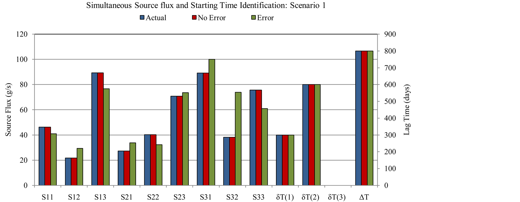
Figure 4. Identification results for Scenario 1.
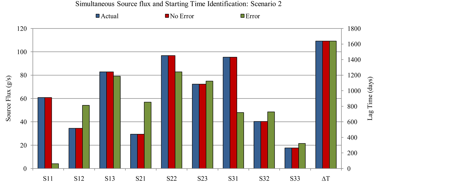
Figure 5. Identification results for Scenario 2.
8. Summary and Conclusions
This developed methodology for simultaneous identification of the source fluxes and their starting time appears to perform satisfactorily in estimating the unknown groundwater pollution source fluxes and their starting times for the illustrative example. These results show that this proposed methodology is capable of overcoming major limitations in the earlier methods. The main limitations of these earlier proposed source identification methods were: 1) It assumed that the starting time of the activity of the sources is precisely known; 2) In scenarios where the time span for the possible start of the sources activities is known with fair degree of certainty, actual starting time was estimated indirectly by solving for source flux magnitudes; 3) In scenarios, where there was no information of the time span for the possible start of the sources activities, solving indirectly for a large number source flux magnitudes over a very large time span, rendered the earlier methods computationally infeasible.
The proposed methodology is applicable to real world problems of source identification in polluted aquifer sites, where no information is available about the starting times of the sources activity and the uncertainty spans over a large time period. This methodology in its current form can estimate the activity starting times for all the potential sources both in steady state and transient conditions. It can also handle multiple sources having different source activity initiation times and missing observation data.
The main advantage of the proposed methodology is its capability to treat the starting time of source activity as an explicit decision variable. This capability has the potential to render many real life unknown groundwater pollution source identification problems computationally feasible. This will ultimately enhance the capability of addressing groundwater pollution remediation issue in complex contaminated aquifer study areas, where there is very little prior knowledge of the source location, source flux release history, and the source activity initiation time.
Acknowledgements
We acknowledge the financial support for this work provided by CRC for Contamination Assessment and Remediation of the Environment (CRC-CARE), Australia and James Cook University, Australia.
References
- Mahar, P.S. and Datta, B. (2000) Identification of Pollution Sources in Transient Groundwater System. Water Resource Management, 14, 209-227. http://dx.doi.org/10.1023/A:1026527901213
- Yeh, W.W.-G. (1986) Review of Parameter Identification Procedure in Groundwater Hydrology: The Inverse Problem. Water Resources Research, 22, 95-108. http://dx.doi.org/10.1029/WR022i002p00095
- Gorelick, S.M., Evans, B. and Ramson, I. (1983) Identifying Sources of Groundwater Pollution: An Optimization Approach. Water Resources Research, 19, 779-790. http://dx.doi.org/10.1029/WR019i003p00779
- Datta, B., Beegle, J.E., Kavvas, M.L. and Orlob, G.T. (1989) Development of an Expert-System Embedding Pattern-Recognition Techniques for Pollution Source Identification. Technical Report, Department of Civil Engineering, California University, Davis.
- Bagtzoglou, A.C., Dougherty, D.E. and Tompson, A.F.B. (1992) Application of Particle Methods to Reliable Identification of Groundwater Pollution Sources. Water Resources Management, 6, 15-23. http://dx.doi.org/10.1007/BF00872184
- Wagner, B.J. (1992) Simultaneous Parameter Estimation and Contaminant Source Characterization for Coupled Groundwater Flow and Contaminant Transport Modeling. Journal of Hydrology, 135, 275-303. http://dx.doi.org/10.1016/0022-1694(92)90092-A
- Woodbury, A.D. and Ulrych, T.J. (1996) Minimum Relative Entropy Inversion: Theory and Application to Recovering the Release History of a Groundwater Contaminant. Water Resources Research, 32, 2671-2681. http://dx.doi.org/10.1029/95WR03818
- Woodbury, A.D., Sudicky, E., Ulrych, T.J. and Ludwig, R. (1998) Three Dimensional Plume Source Reconstruction Using Minimum Relative Entropy Inversion. Journal of Contaminant Hydrology, 32, 131-158. http://dx.doi.org/10.1016/S0169-7722(97)00088-0
- Mahar, P.S. and Datta, B. (1997) Optimal Monitoring Network and Ground-Water Pollution Source Identification. Journal of Water Resources Planning and Management, 123, 199-207. http://dx.doi.org/10.1061/(ASCE)0733-9496(1997)123:4(199)
- Mahar, P.S. and Datta, B. (2001) Optimal Identification of Ground-Water Pollution Sources and Parameter Estimation. Journal of Water Resources Planning and Management, 127, 20-29. http://dx.doi.org/10.1061/(ASCE)0733-9496(2001)127:1(20)
- Sidauruk, P., Cheng, A.H.-D. and Ouazar, D. (1997) Ground Water Contaminant Source and Transport Parameter Identification by Correlation Coefficient Optimization. Ground Water, 36, 208-214. http://dx.doi.org/10.1111/j.1745-6584.1998.tb01085.x
- Skaggs, T.H. and Kabala, Z.J. (1994) Recovering the Release History of a Groundwater Contaminant. Water Resources Research, 30, 71-79. http://dx.doi.org/10.1029/93WR02656
- Liu, C. and Ball, W.P. (1999) Application of Inverse Methods to Contaminant Source Identification from Aquitard Diffusion Profiles at Dover AFB, Delaware. Water Resources Research, 35, 1975-1985. http://dx.doi.org/10.1029/1999WR900092
- Skaggs, T.H. and Kabala, Z.J. (1995) Recovering the Release History of a Groundwater Contaminant Plume: Method of Quasi-Reversibility. Water Resources Research, 31, 2669-2673. http://dx.doi.org/10.1029/95WR02383
- Bagtzoglou, A.C. and Atmadja, J. (2003) Marching-Jury Backward Beam Equation and Quasi-Reversibility Methods for Hydrologic Inversion: Application to Contaminant Plume Spatial Distribution Recovery. Water Resources Research, 39, 10-14.
- Atmadja, J. and Bagtzoglou, A.C. (2001) Pollution Source Identification in Heterogeneous Porous Media. Water Resources Research, 37, 2113-2125. http://dx.doi.org/10.1029/2001WR000223
- Bagtzoglou, A.C. and Baun, S.A. (2005) Near Real-Time Atmospheric Contamination Source Identification by an Optimization-Based Inverse Method. Inverse Problems in Science and Engineering, 13, 241-259. http://dx.doi.org/10.1080/10682760412331330163
- Aral, M., Guan, J. and Maslia, M. (2001) Identification of Contaminant Source Location and Release History In aquifers. Journal of Hydrologic Engineering, 6, 225-234. http://dx.doi.org/10.1061/(ASCE)1084-0699(2001)6:3(225)
- Mahinthakumar, G. and Sayeed, M. (2005) Hybrid Genetic Algorithm-Local Search Methods for Solving Groundwater Source Identification Inverse Problems. Journal of Water Resources Planning and Management, 131, 45-57. http://dx.doi.org/10.1061/(ASCE)0733-9496(2005)131:1(45)
- Singh, R.M. and Datta, B. (2006) Identification of Groundwater Pollution Sources Using GA-Based Linked Simulation Optimization Model. Journal of Hydrologic Engineering, 11, 101-109. http://dx.doi.org/10.1061/(ASCE)1084-0699(2006)11:2(101)
- Singh, R.M. and Datta, B. (2004) Groundwater Pollution Source Identification and Simultaneous Parameter Estimation Using Pattern Matching by Artificial Neural Network. Environmental Forensics, 5, 143-159. http://dx.doi.org/10.1080/15275920490495873
- Singh, R.M. and Datta, B. (2007) Artificial Neural Network Modeling for Identification of Unknown Pollution Sources in Groundwater with Partially Missing Concentration Observation Data. Water Resources. Management, 21, 557-572. http://dx.doi.org/10.1007/s11269-006-9029-z
- Singh, R.M., Datta, B. and Jain, A. (2004) Identification of Unknown Groundwater Pollution Sources Using Artificial Neural Networks. Journal of Water Resource Planning and Management, 130, 506-514. http://dx.doi.org/10.1061/(ASCE)0733-9496(2004)130:6(506)
- Datta, B., Chakrabarty, D. and Dhar, A. (2009) Optimal Dynamic Monitoring Network Design and Identification of Unknown Groundwater Pollution Sources. Water Resources Management, 23, 2031-2049.
- Datta, B., Chakrabarty, D. and Dhar, A. (2009) Simultaneous Identification of Unknown Groundwater Pollution Sources and Estimation of Aquifer Parameters. Journal of Hydrology, 376, 48-57.
- Datta, B., Chakrabarty, D. and Dhar, A. (2011) Identification of Unknown Groundwater Pollution Sources Using Classical Optimization with Linked Simulation. Journal of Hydro-Environment Research, 5, 25-36. http://dx.doi.org/10.1016/j.jher.2010.08.004
- Azghadi, B.N.S., Kerachian, R., Lari, M.R.B. and Solouki, K. (2010) Characterizing an Unknown Pollution Source in Groundwater Resources Systems Using PSVM and PNN. Expert Systems with Applications, 37, 7154-7161. http://dx.doi.org/10.1016/j.eswa.2010.04.019
- Bagtzoglou, A.C. (2003) On the Non-Locality of Reversed Time Particle Tracking Methods. Environmental Forensics, 4, 215-225. http://dx.doi.org/10.1080/713848511
- Ababou, R., Bagtzoglou, A.C. and Mallet, A. (2010) Anti-Diffusion and Source Identification with the RAW Scheme: A Particle-Based Censored Random Walk. Journal of Environmental Fluid Mechanics, 10, 41-76. http://dx.doi.org/10.1007/s10652-009-9153-4
- Ayvaz, T.M. (2010) A Linked Simulation-Optimization Model for Solving the Unknown Groundwater Pollution Source Identification Problems. Journal of Contaminant Hydrology, 117, 46-59. http://dx.doi.org/10.1016/j.jconhyd.2010.06.004
- Jha, M.K. and Datta, B. (2011) Simulated Annealing Based Simulation-Optimization Approach for Identification of Unknown Contaminant Sources in Groundwater Aquifers. Desalination and Water Treatment, 32, 79-85. http://dx.doi.org/10.5004/dwt.2011.2681
- Prakash, O. and Datta, B. (2012) Sequential Optimal Monitoring Network Design and Iterative Spatial Estimation of Pollutant Concentration for Identification of Unknown Groundwater Pollution Source Locations. Environment Monitoring Assess, 185, 1-8. http://dx.doi.org/10.1007/s10661-012-2971-8
- Chadalavada, S., Datta, B. and Naidu, R. (2011) Optimisation Approach for Pollution Source Identification in Groundwater: An Overview. International of Environment and Waste Management, 8, 40-61. http://dx.doi.org/10.1504/IJEWM.2011.040964
- Amirabdollahian M. and Datta, B. (2013) Identification of Contaminant Source Characteristics and Monitoring Network Design in Groundwater Aquifers: An Overview. Journal of Environmental Protection, 4, 26-41. http://dx.doi.org/10.4236/jep.2013.45A004
- Atmadja, J. and Bagtzoglou, A.C. (2001) State of the Art Report on Mathematical Methods to Reliable of Groundwater Pollution Source Identification. Environmental Forensics, 2, 205-214. http://dx.doi.org/10.1006/enfo.2001.0055
- Bagtzoglou, A.C. and Atmadja, J. (2005) Mathematical Methods for Hydrologic Inversion: The Case of Pollution Source Identification. Chapter in Environmental Impact Assessment of Recycled Wastes on Surface and Ground Waters. In: Kassim, T.A., Ed., Engineering Modeling and Sustainability, The Handbook of Environmental Chemistry, Water Pollution Series, Vol. 3, Springer-Verlag, Heidelberg-New York, Vol. 5, Part F, 65-96.
- Harbaugh, A.W., Banta, E.R., Hill, M.C. and McDonald, M.G. (2000) MODFLOW-2000, the US Geological Survey Modular Ground-Water Model. US Geological Survey Open-File Report 00-92, US Geological Survey, Reston.
- Rushton, K.R. and Redshaw, S.C. (1979) Seepage and Groundwater Flow. Earth Surfaces Processes, 5, 339.
- Zheng, C. and Wang, P.P. (1999) MT3DMS: A Modular Three-Dimensional Multi-Species Transport Model for Simulation of Advection, Dispersion and Chemical Reactions of Contaminants in Groundwater Systems. US Army Engineer Research and Development Center Contract Report SERDP-99-1, Vicksburg.
- Domenico, P.A. and Schwartz, F.W. (1998) Physical and Chemical Hydrogeology. 2nd Edition, John Wiley & Sons, Inc., New York.
- Kirkpatrick, S., Gelatt, D.C. and Vecchi, P.M. (1983) Optimization by Simulated Annealing. Science Magazine, 220, 671-680. http://dx.doi.org/10.1126/science.220.4598.671
- Metropolis, N., Rosenbluth, A., Rosenbluth, M., Teller, A. and Teller, E. (1953) Equation of State Calculations by Fast Computing Machines. Journal of Chemical Physics, 21, 1087-1092. http://dx.doi.org/10.1063/1.1699114
- Datta, B., Prakash, O., Campbell, S. and Escalada, G. (2013) Efficient Identification of Unknown Groundwater Pollution Sources Using Linked Simulation-Optimization Incorporating Monitoring Location Impact Factor and Frequency Factor. Water Resources Management, 27, 4959-4976.
Notation
The following symbols are used in this paper:
NOTES

*Corresponding author.