ABSTRACT

It was not until the end of the 1990’s that animal born satellite receivers catapulted range cattle ecology into the 21st century world of microchip technology with all of its opportunities and challenges. With the global navigation satellite system (GNSS), insight about how cattle use a landscape is being revealed from previously unknown temporal and spatial behaviors. The most common system to date for studying ungulate movement is the global positioning system (GPS). With its use has come a clarity and completeness in documenting spatial and temporal data in new and exciting ways that offer almost unlimited possibilities to better understand and manage economic and societal returns from animal dominated landscapes. However, its use on free-ranging cattle is not without challenges, some of which are yet to be optimally solved. To maximize the usefulness of GNSS data, consideration must be given to: 1) developing a standardized protocol for reporting and analyzing research that facilitates interpretation of results across different ecosystems; 2) develop optimum ranges over which to collect satellite fixes depending upon the particular behaviors of interest; and 3) concurrently develop electronic hardware and equipment platforms that are easily deployed on animals and that are light, robust, and can be worn by cattle for extended periods of time without human intervention (e.g., changing batteries). Once data are collected, appropriate geographic information system (GIS) based models should be used to produce a series of products that can be used to implement flexible management strategies, some of which may support methodologies that are yet to be commercialized and adopted into future plant-animal interface management routines.

1. Introduction

Free-ranging animal behavior is challenging to study and manage in light of the more than 68 factors that have been shown to influence it [1]. Obtaining both accurate and precise cattle behavior data is essential to understand and subsequently manage free-ranging animals. Of the 40 different behaviors cattle can engage in [2], 95% of them can be classified into one of four main activities: foraging, walking, standing, or lying [3]. Foraging is probably of greatest interest to most land stewards because of the impact it has on animal dominated landscapes, especially when these landscapes are required to supply goods and services beyond providing adequate nutrition for free-ranging animals. Therefore, studying animal-to-animal variability is basic to understanding free-ranging animal behavior [4].

The official study of animal behavior did not become part of agricultural college curricula until the late 1950’s [5]; however, the importance of behavior was recognized in husbandry texts dating back to the 1800’s [6]. Focused livestock behavior research in the USA began in the 1920’s. Early studies such as those of Sheppard [7] and Cory [8] relied entirely on eyesight and hand written recordings to document the behaviors observed. Thereafter, sight and stop-watches remained the sole tools for documenting free-ranging animal behavior for many years [9]. Today observation still remains a powerful and useful tool for documenting free-ranging animal behavior [10- 16]; however, it has limitations especially during periods of darkness [3] and following extended periods of continuous observation when fatigue can accentuate observer bias [17]. Furthermore, the mere presence of an observer can impact both wildlife [18] and domestic animal [19,20] behaviors. The question then becomes “how is the observer influencing the observation?” The answer to this question is not trivial and frequently is not provided by researchers who do not describe protocols to minimize its potential bias in behavioral studies [21].

Various techniques have been employed to improve observation accuracy by reducing the distance between an observer and the animal being observed. Observing from parked vehicles [22], horseback [23] or platforms positioned above the ground [24] have been used. Though sampling methods exist for observational data [25], there is as yet no tool available that can overcome human inefficiency when multitasking [26], a prerequisite for observing and recording data from more than one animal at a time.

Furthermore, to overcome human sight limitations, binoculars [27] as well as night vision technologies [28, 29], video recordings [30] and even lasers [31] have been employed. As early as the 1950’s, electronics were used to track wildlife [32]. Because of their lead, wildlife researchers established many of the guidelines used throughout the 20th century for tracking domestic animals. One of the earliest attempts to augment observations of cattle behavior with electronics was a biotelemetry system developed by Australian researchers in the 1970’s [33]. For a complete discussion of electronics in wildlife tracking the reader is directed to texts by Kenward [34] and Millspaugh and Marzluff [35]. Currently no textbooks exist to assist range-animal ecologists in developing protocols for monitoring free-ranging livestock using 21st century technologies. This review traces the application of the global navigation satellite system (GNSS) [36,37] for tracking free-ranging cattle with a focus on its implementation and the challenges range animal scientists face when deploying GNSS to study free-ranging cattle behaviors.

2. A Satellite Based Technology

The GNSS can be traced back to 1966 as described in the Woodford/Nakamura Report [38,39]. Of the several satellite-based systems being used or developed today [40, 41]; (see Table 1) the most familiar tracking system is the NAVigation Satellite Timing And Ranging (NAVSTAR) System [42] commonly referred to as the global positioning system (GPS) [43].  

Contrary to some versions of GPS, this utility was developed initially for both military and civilian users [37]. The technology is robust with respect to electric transmission lines [44] yet GPS signals are very weak at the surface of the earth making them susceptible to interference and jamming [45] as well as potentially being vulnerable to spoofing [46].

Research using GPS-based telemetry systems for tracking animals began in 1991 [47]. Six years later, cows were monitored for the first time using this technology [48]. Since 1997, at least 99 studies have been reported in which GNSS devices have been used to monitor free-ranging cattle behavior (Table 2). Being able to characterize animal behavior data within a spatial as well as a temporal context with respect to peers and the landscape is a major benefit provided by GNSS data [16,49]. In addition to monitoring spatial and temporal information, GNSS technology has been combined with other electronics to monitor free-ranging animal health [50] and numerous other behaviors associated with foraging and moving [51]. Most studies employing GNSS have attached the devices directly to the free-ranging animal; however, cows can be successfully tracked by a person moving with cattle that carries a GPS unit [52- 54].

3. GNSS Devices

Applying GNSS technology to free-ranging animals is expensive and remains a major challenge when designing studies to track free-ranging cattle [56]. A sheep was the first domestic ruminant on which a GNSS device was deployed at a cost exceeding $47,000 per unit in 2011 US dollars [55]. The first commercially available GPS units could cost between $2500 and $5000 [47]. In 2012 the price of individual GNSS devices ranged between $500 and >$3000 per animal, with low cost units typically being non-commercial tracking devices not specifically designed for tracking animals [57].

Most biologists/ethologists and technicians are not skilled in reading electronic schematics or performing electronic assembly, let alone attending to electronic maintenance. However, for those with this expertise on their team and 4 to 5 hours of time that can be devoted to build a GNSS tracking device, the Clark animal tracking system (ATS) [58] may be the most user friendly package currently available, since a detailed bill of materials is available at http://clark.nwrc.ars.usda.gov/collars/. Other hand built GNSS tracking devices have been described in the literature [57,59] but instructions for their assembly are less detailed than that provided for the Clark ATS. An alternative to purchasing devices specifically built to track free-ranging animals is to purchase a commercial GNSS device designed for recreational purposes that can be attached to an equipment platform designed to be worn by free-ranging animals. Several researchers [30,48,57,60-67] have adapted various models of Garmin GNSS products while the Magellan 315 has also been successfully used [68]. Several researchers have also used GNSS devices incorporated into electronic systems manufactured either by individuals [69] or university departments or research organizations with electronic/computer engineering expertise [16,70-81]. For those who choose to use commercial equipment designed specifically for free-ranging animals, a number of companies are listed on the World Wide Web. To date, the company whose products have been used most often to monitor cattle (Table 2) is headquartered in Newmarket, Ontario Canada. Lotek began manufacturing equipment for tracking wildlife in 1984 and by 1995 touted the world’s first automatic large mammal tracking system

Table 1. The global navigation satellite system (GNSS).

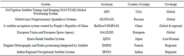
based on GNSS technology [82].

One of the greatest advantages of on-site assembly of GNSS devices vs. commercial products is reduced “downtime” during equipment failure. When commercial equipment fails, it normally cannot be repaired on site and must be returned to the manufacturer. This can interfere with data collection. One method to address equipment failure is to have back-up units available for deployment when GNSS devices fail. Though it increases the initial cost of a project, this approach seems reasonable; yet none of the studies reported in Table 2 specifically indicated this was a part of their experimental protocol.

Though GNSS equipment failure may not occur when devices are deployed on free-ranging animals [83], this is the exception rather than the rule (see Table 2). Future GNSS animal tracking manuscripts should publish failure rates as well as reasons or suspected reasons for failure. This information will assist future behavior-based GNSS research to develop protocols that can minimize data loss as well as providing information useful to commercial companies seeking to manufacture more robust models of their equipment [42,84]. Resolving equipment failures quickly is important because incomplete GNSS data sets result in poor statistical inferences [85]. However, it has been suggested that GNSS data sets with <10% missing data can be safely analyzed to determine habitat-selection [86].

4. Number of Cattle to Instrument

No studies to date have been conducted to determine exactly how many animals within a group need to be instrumented to accurately describe the group behavior being investigated. Differences exist even among identical twin dairy cattle [4] so it is no surprise that more than one GPS instrumented animal is needed to accurately describe behaviors such as grazing within a group of cattle [87]. Animal to animal variability exists in wildlife species [88] as well as domestic cattle [12] and this variability may be quite large depending on the individual animal behaviors of interest. Therefore, research is needed to determine what percentage of a herd should be instrumented to accurately describe herd behavior [79]. Cattle behave gregariously in groups, which has been cited as justification for instrumenting only a few animals [89]; however, very large discrepancies in behavior among individual(s) within a herd have been reported [49]. The problem of adequate sample size has been exacerbated by satellite tracking technology because of the expense of GNSS units [90]. Though determining number of animals to instrument will probably always be linked to cost and though a sample size of 6 to 12 subjects should be considered low, this number may be suitable for well-planned experiments based on correlational evidence [91]. As few as four steers grazing a 0.16 ha irrigated paddock were able to accurately categorize grazing, ruminating and idling with observation periods between 15 and 30 minutes [92]. Management recommendations regarding watering location have been advocated based on GNSS data from only two cows [93]. However, it is safe to assume that most foraging animals only behave “normally” when held in groups [94].

Significant error can be introduced by characterizing landscape utilization patterns with data from only a few animals. Location errors were found to increase from 10% when four of five cows were used in a model to 40% when only a single cow was used [49]. Therefore, it might be concluded that many of the studies in Table 2 may have had too few animals instrumented to provide an accurate picture of herd activity. Activity sensor output from a single collar was found not to be reliable for classifying behaviors into grazing, travel and resting using 5-min intervals between GPS fixes and furthermore, lying could not be separated from standing [94]. However, the shorter the interval between fixes, the less problem there is in discriminating among behaviors. Foraging, walking, and stationary behaviors of four cows were successfully characterized using rate of travel based on uncorrected GNSS fixes recorded at 1 s intervals [16]. However, increased frequency of fix rate increases power

Table 2. Ranking of 99 free-ranging cattle studies beginning in 1997 through 2012 that have employed global navigation satellite system (GNSS) technology. Blank cells indicate data not provided by the author(s) and could not be calculated from manuscript.

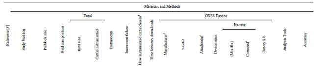
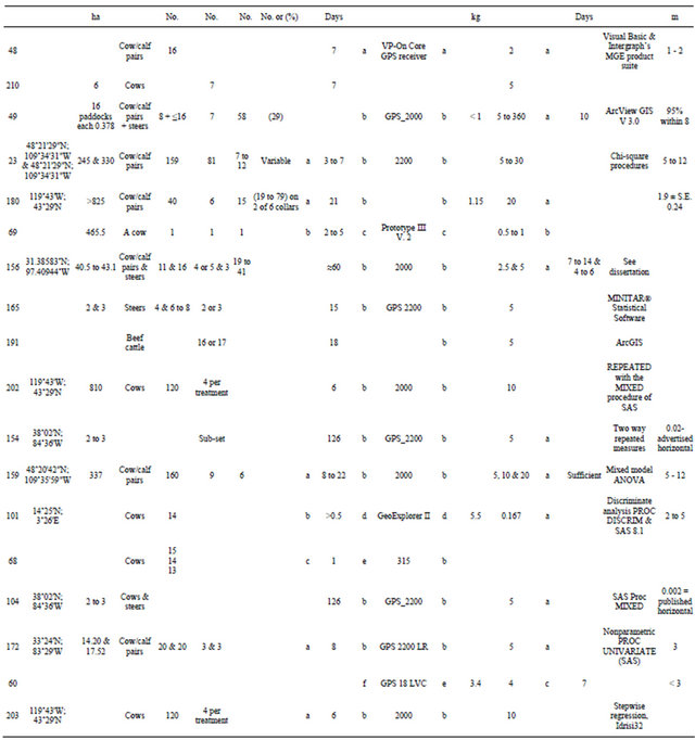
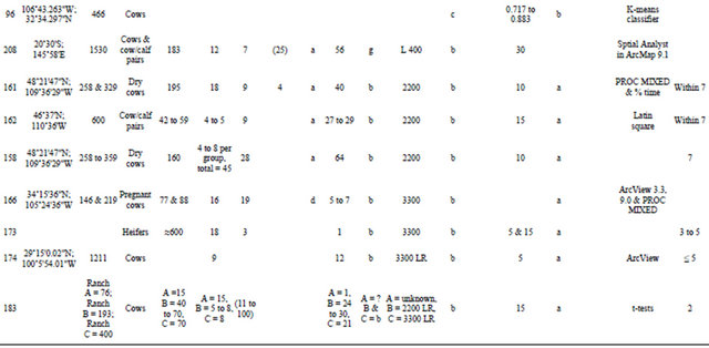
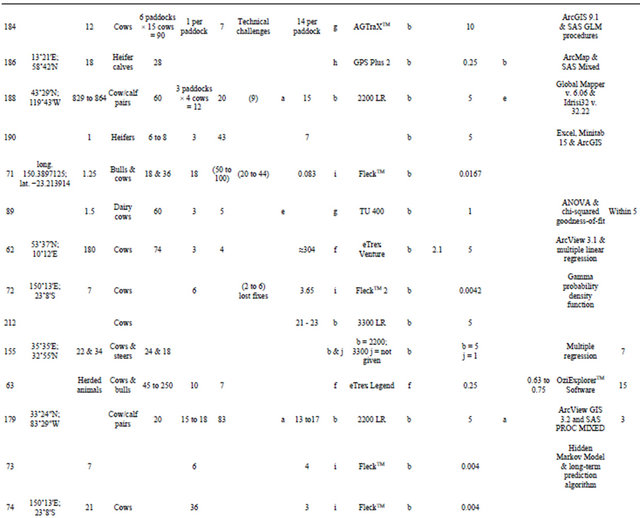
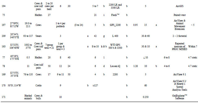
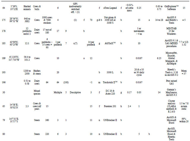
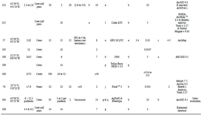
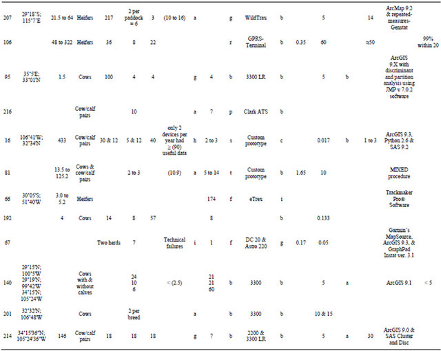
¹How instrumented cattle chosen: a = Randomly; b = Selected; c = Lead cow; d = Availability; e = Carefully chosen; f = Chute cut; g = Not random; h = Docile disposition; i = Based on leadership; ²Manufacturer: a = Motorola; b = Lotek; c = Future Segue; d = Trimble; e = Magellan; f = Garmin^TM; g = Blue Sky Telemetry^TM; h = Vectronie-Aerospace GmbH; i = CSIRO; j = Trilogical; k = Wildlife Track Inc.; l = Custom; m = Telespial Systems; n = University of New England; o = ATF Co. Ltd.; p = Televilt; q = Ames Laboratory; r = Telespor; s = MIT Computer Science and Artificial Intelligence Lab; t = Engineering Services Group; ³Attachment: a = Hand-made girth harness; b = Neck collar; c = Neck Saddle; d = Canvas backpack; e = Shoulder harness; f = Handmade collar taped to cowbell; g = Harness; h = Girth Strap; i = Halter mount; ⁴Fix rate corrected: a = DPGS; b = None; C = WAAS; d = EGNOS; e = Lotek N4 v.1.1895 software.

requirements but the number of location fixes recorded per unit of time can be reduced with software that will “power down” the electronics when animals are not moving [96]. Recently a hybrid system was developed that employs a kinetically powered network of primary and secondary nodes powered by the movement of an animal’s neck. When these systems are combined with GPS technology at specific locations, termed “hotspots”, autonomous monitoring of free-ranging animals (reindeer were the test subjects) may be economically feasible over landscapes ≤ 2000 km² [97]. Future GNSS studies to determine the correct ratio of instrumented to non-instrumented animals required to accurately characterize the behavior of interest among various landscapes are needed.

5. Methods of Attaching GNSS Devices to Cattle

Recommendations exist regarding the maximum percentage of an animal’s mass equipment platforms can be without negatively affecting behaviors [98]; however, relatively lightweight wildlife collars can have activity specific impacts even at <1% of the animal’s total body mass [99]. Using a collar that does not exceed a certain percentage of an animal’s body mass may be a good rule of thumb, but it is critical that animal behavior not be adversely changed by the equipment package [100,101]. Such knowledge can only be gained by diligent observation of animals on the landscape in which they are to be monitored prior to instrumentation. Though lag time recommendations have not been specifically reported for cattle, GNSS data collection should be delayed at least a few hours following instrumentation to allow animals to adjust to the equipment. Again observation of the animal after it is instrumented is necessary to determine the optimum time necessary for each animal’s personality to accept wearing the equipment package. In sheep a 16 h period between instrumenting an animal and the onset of data collection appears to be adequate [102].

Regardless of the GNSS device used, the predominant method employed for deploying GNSS devices on cows has been neck collars (Table 2). However, girth harnesses or backpacks [48] and various shoulder harness platforms have also been used [57,60,61,65,66,101,103]. Each equipment platform design has its own merits as well as challenges. Equipping cows with neck collars is an art in terms of placing the correct tension on the collar. If the tension is too tight, skin abrasion can occur, but a loose collar may slide over the cow’s head during grazing or get caught on objects in the landscape. Furthermore, tension can affect the data quality if the electronics package contains motion sensors capable of measuring side-to-side and/or up and down movement of the head and neck [104]. Mounting “differences” have been found to affect sensor counts among collars [49]; this suggests a protocol be developed for calibrating individual collars. Magnetometer signals can differ based on hardware orientation [51]. To address proper collar tension on cattle it may be possible to use a neck collar composed of elastic material that would stretch yet remain tight during deployment to eliminate skin abrasion yet prevent slippage. In a stretch design the belt material would have to be capable of wicking sweat and moisture away from the animal’s skin to minimize abrasion. An adjustable slip noose collar has been designed for use on domestic lambs and several wildlife species [105].

If a collar rotates such that the GNSS antenna is not pointed skyward, GNSS fixes can be lost [24,70]. Even though some non-skyward orientations of antennas may allow GPS fixes to be captured, it will be less efficient [106]. Most collar designs position the heaviest components (usually the batteries) on either side of the neck to act as counter balances [24,70] or allow batteries to freely slide on a belt as the battery hangs below the animal’s neck [16] to help stabilize the GNSS antenna in a skyward position. Another technique to help keep the GPS antenna pointed skyward has been to attach a dense foam rubber pad in the shape of an open “V” to the top of the equipment box hanging below the cow’s neck to prevent rotation [77]. When the collar is adjusted to the proper tension, the cow’s neck fits into this “V” and reduces the tendency of the collar to swing from sideto-side or rotate. The combination of head halters with wide neck belts or saddles has also been used successfully to deploy GPS antenna on free-ranging cattle [16, 24,107].

The use of GPS tags in wildlife research [91], termed bio-logging [108], is increasing and packaging GNSS into ear tags for use on free-ranging cattle is currently being advertised as a commercial reality. Reducing energy consumption [109], the need to reduce battery mass [110] of an ear tag, and designing an antenna that is robust and always able to receive the GNSS signal [111] are just three of the challenges. The earliest attempts to place electronics in ear tags to be worn by cattle were not successful because the studs used to attach a 113 g tag to the cattle’s ear pinna were too short and caused abrasion; however, by increasing the stud length to 3.81 cm and drilling holes through the nylon washer that held the ear tag in place, ear damage was eliminated [112]. More recent research found ear tags weighing between 227 g and 250 g could only be tolerated for three to five days if placed close to a cow’s head [110]. Reducing the mass and increasing length of the button studs allowed feedlot cattle to tolerate a 114 g tag for up to four weeks. However, for long term deployment ear tags should probably not exceed 25 g [112].

6. Accuracy or Precision

Accuracy is not a fundamental characteristic of a dataset but must be derived from outside itself; therefore, collecting more GNSS data may not necessarily improve accuracy but could actually decrease accuracy [113]. Furthermore, differential correction of GPS data (DGPS) also contains errors with accuracy degrading at an approximate rate of 1 m for each 150 km distance the GPS unit is from the reference station [114]. Not only do methods for correcting GNSS data differ [115] but static and dynamic accuracies differ [116,117].

It is ironic that most free-ranging animal studies in which GNSS data are collected focus on the temporal and spatial data of moving cattle yet accuracy figures reported by most researchers refer to static accuracy (Table 2). Furthermore, not all collars, even from the same manufacturer and model, have identical accuracy when tested statically or dynamically, and it is not uncommon to find a manufacturer’s reported accuracies stated in published research without providing the statistical basis for the stated accuracy [118]. Since location error is affected by vegetation [119], topography (especially in conjunction with canopy cover) [120] and animal behavior, these factors need to be evaluated prior to deployment of GNSS devices on free-ranging animals [121]. Evaluating GNSS devices before deployment is critical because each device has inherent differences, including fix rate at a given setting, causing variation among individual devices [79,118,122]. A set logging interval of 15 s can result in 2.3 to 3.8 fixes per minute (P < 0.001) depending on landscape terrain/obstructions, yet differences in open terrain were negligible [123]. Measures of accuracy can be means or counts and accuracy specifications should always state the metric used. This relationship is complex because GNSS positions exist in three dimensions yet knowing most locations in 2D (a flat map) is adequate [124] (Table 3).

However, if 3D information is desired, then root mean square (rms) vertical, twice the distance of the root mean square (2drms) or spherical error probable (SEP) would be a more appropriate set of statistics to consider. Most often when accuracy is stated (e.g. 5 m), it is most likely a circular error probability (CEP) which assumes GNSS errors are Gaussian and have a circular distribution [124]. However, the shape of error distributions is a function of how many satellites are being tracked and where they are located in the sky. A more circular error pattern occurs when more satellites are in view, whereas fewer satellites create a more elliptical pattern and a corresponding higher horizontal dilution of precision (HDOP). Both autonomous and differential global positioning system (DGPS) errors are approximately Gaussian, but because GNSS errors are correlated in time, a stationary receiver will produce errors that for one period of time may tend to be in one direction and at a later period of time may be in a different direction [124]. This is because the GNSS signal is non-stationary [113]. The positional dilution of precision (PDOP) is based on the number as well as the geometry of the satellites available to the GNSS device; the lower the PDOP number, the more accurate the GPS fix. As more satellite systems (Table 1) [36,125] come on line, the error distributions will become more circular [124] which will benefit data accuracy and analyses. Furthermore, GNSS users who require real-time data will benefit from receivers using both GPS and GLONASS data to lower PDOP. Using both GPS and GLONASS at mid-latitudes can lower PDOP more than 15% and at latitudes above 55˚ PDOP could be lowered by as much as 30% using both systems [41].

Unfortunately, many authors use precision and accuracy interchangeably when discussing GNSS though statistically they are distinctly different. Today we can track animals with a precision never before possible using GNSS [42]; however, determining GNSS accuracy remains largely undocumented or possibly inappropriately documented. The GNSS devices used in the studies listed in Table 2 usually either restated accuracy provided by the manufacturer (most likely a static accuracy) or restated accuracy cited in previous research using the same model GNSS device. Only a few researchers have attempted to determine GNSS accuracy of their devices [118,122,126] and it was static accuracy they evaluated and unfortunately static and dynamic accuracy are different [117]. Furthermore, most commercial suppliers provide only static accuracy values [127]. The static accuracy of GNSS devices has been reported to be between 0.01 m [128] and 15 m [129]. On May 2, 2000 at 12:00 AM when selective availability was deactivated, accuracy of GPS data improved substantially [130] and together with differential correction location error has now been decreased from 80 m to 4 m [131]. Earlier methods

Table 3. Global Navigation Satellite System (GNSS) measures of horizontal accuracy in meters and their relationship for circular, Gaussian, and error distributions (adapted from [124]).

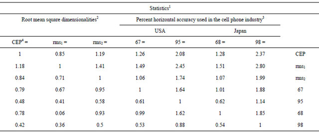
¹How to make conversions using this table. Horizontal statistics are the product of multiplying the vertical statistics by the appropriate cell value; an example: rms₂ = rms₁ × 1.41; ²The square root of the one dimensional mean rms₁ or North error and for rms₂, the horizontal error representing the square root of the mean of the squared horizontal error; 2 drms is twice the horizontal rms, i.e., 2 drms = 2 × rms₂; ³Refers to the radii of circles, centered at the antenna position containing between 67 and 98 percent of the points in a scatter plot; ⁴Circular Error Probable (CEP) refers to the radius of a circle, centered at the antenna position, containing 50% of the points in a scatter plot. It should NEVER be associated with another percentage.

that employed triangulation of Very High Frequency (FHV) radio signals were in the range of 70 to 600 m [126,132]. Reporting only the static accuracy of GNSS devices is not totally correct since the major reason for instrumenting cattle with GNSS devices is to improve our understanding of their dynamic behaviors [133]. Furthermore, stationary collars may be as much as 33% more successful at acquiring fixes than when deployed on animals [134].

Though literature exists that describes how dynamic testing of GNSS devices can be accomplished [116,117], the testing of GNSS devices to be deployed on cattle using this equipment will probably not be possible for most ethologists. This quandary may have a relatively simple solution. One approach would be to “etch” a pattern into the soil surface or place something on the surface that could be followed to delineate a pattern with straight and curved segments (similar to a typical cattle route). This pattern could be replicated in any ecosystem for evaluating dynamic aspects of GNSS devices. The length of this pattern would be based on the number of GNSS fixes per unit of time. The devices could be carried along the route either on foot or by an all-terrain vehicle at a realistic walking speed for moving cattle (e.g. ≤3.2 km/hr; 2 miles/hour). This speed can be used to gather cattle on the Jornada Experimental Range and probably represents a maximum walking rate of travel for cattle except for brief periods when they may run for very short distances. The number of times required to traverse the route would depend on a number of factors, especially those influenced by the geometry of the satellites in the sky and the rate at which GNSS fixes were being recorded. If tree cover is a concern when actual data collection takes place, tests should be performed under both open and closed canopies. This protocol would provide a measure of dynamic instrument-to-instrument precision among the devices to be deployed on free-ranging animals. Furthermore, it would be possible to calculate each instrument’s dynamic accuracy by comparing the instrument’s data to data obtained using survey grade GPS equipment to document the path’s spatial location on the landscape.

Recent publications suggest the dynamic behaviors of walking and foraging by cattle can be determined at GNSS fix rates of <5 min [16,72,101]. Currently this is a concern because most commercial GNSS devices have a maximum fix rate of ≥5 min (Table 2). The reason for the 5 min maximum fix rate among many commercially available GNSS units for free-ranging animals is unclear but most likely arose from the inability of wildlife researchers to easily recapture animals to change batteries and/or download data stored in memory. The need for an increased GNSS fix rate for livestock studies may change this industry norm. In the future it may be possible to deploy GNSS devices for longer periods by using solar [107,135] or kinetic [136] energy to recharge batteries, though this is not presently a commercially practical reality. Furthermore, data storage, once a challenge, is of little concern today due to the ability to periodically wirelessly transmit data back to a base station or to store data on the animal using memory cards with substantial memory [135].

7. GNSS Data, Maps and Analysis

The intent of this review is not to delve into the intricacies of combining GNSS data with geographical Information systems (GIS) data. However, scale and resolution must be considered when designing research involving GNSS data. If GNSS data are to be plotted on maps it is currently possible to purchase aerial satellite photography with spatial resolution of 300 mm and with images available in a number of spectral bands (Table 4). If satellite spatial resolution is not adequate, cameras fixed to remote controlled helicopters [137] or unmanned aerial vehicles [138] can produce images with 1 mm and 30 to 60 mm resolution, respectively. The key is to determine the scale necessary to evaluate the GNSS data required to answer the question(s) being addressed and to then plan research protocols accordingly.

Currently there is no off-the-shelf solution that combines GNSS data with a GIS package, thus supporting the need for providing adequate methodology detail [139]. One of the most important uses of GNSS data is to guide a researcher’s interpretation of what has taken place on a landscape. Yet there remains a scale-dependence of movement behavior that requires further refinement [85].

Analysis of GNSS data after collecting it may be the most poorly addressed aspect when using GNSS technology to monitor free-ranging cattle behavior. The following example helps to focus on this challenge. Prior to analysis of GPS cow data to address preand postweaning foraging, walking and standing a questionnaire was mailed to colleagues representing the following disciplines: animal science, computer science, computer engineering, ecology, GIS, modeling, range science, robotic engineering and statistics asking them to suggest how the data should be analyzed and why they recommended the tool(s) they did [16]. Of the 45 returned responses (n = 132), 28 different opinions were offered regarding the most appropriate approach for analysis.

The range of opinions received was not surprising but what was surprising was the fact that 11 of 28 statistical approaches suggested were not because the statistics were necessarily the most robust but because respondents were most familiar with them. Since a number of geospatial methods exist for analyzing GNSS data [1], the re-

Table 4. The spectral bands and resolution possible from various commercially available satellite images.

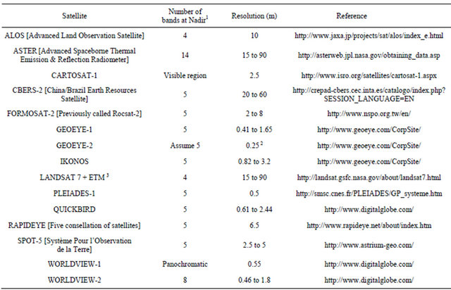
¹The point on the celestial sphere that is located 90˚ directly below the observer; ²Currently the highest commercial resolution allowed by US regulations is 0.5 m or 19.5 inches ground resolution; ³Sensing takes place among seven bands: Aster, Long-wave infrared or thermal IR = 8.125 to 11.650 µm and Landsat-7, Band 6 = 10.4 to 12.5 µm, Band 7 = 2.09 to 2.35 µm, and Band 8 = 0.52 to 0.9 µm.

sults from this questionnaire suggest that guidelines need to be developed to ensure that optimal analyses of geospatial data from GNSS are employed in future animal tracking studies. This may require adding a geospatial statistician to the team at the onset of the study. This is especially important since successive Euclidean distances are significantly correlated when time intervals between successive fixes were <120 m [140]. Here sequential observations are not independent in time or space but are autocorrelated; therefore, movement rates should be evaluated in terms of temporal autocorrelated functions [141]. Probably one of the best analytical approaches for analyzing GNSS data is to sample at the most frequent rate possible and then subsample data over longer intervals if autocorrelation is of concern with the particular statistics being used [140].

8. Implications

Some of the published literature on tracking free-ranging cattle using GNSS technology is noticeably incomplete and does not provide adequate information to replicate the study or accurately apply the findings to animal husbandry practices (see Table 2). To correct this deficiency it is essential that those who use GNSS understand its capabilities as well as its limitations. By addressing these ambiguities experimental protocols will be more complete. The result will be experimental protocols that can be easily adapted or modified when applied to new locations and will result in information pertinent for managing animal dominated landscapes. Because tracking cattle using GNSS technology is still evolving, it would be prudent to set some minimum standards for reporting all future GNSS protocols in which free-ranging animals are to be monitored. At a minimum the standards should include the following information:

• State the geographical coordinates where the study was conducted.

• Specify the datum used to manipulate the raw or corrected fixes.

• Identify number and kind of GNSS devices deployed and the particular fix rate chosen.

• Provide information on the dynamic accuracy of the devices deployed.

• Describe how and why particular animals were chosen for instrumentation.

• Furnish reasons for the particular ratio of instrumented to non-instrumented animals.

• Discuss “equipment death” and the factor(s) causing the devices to fail.

• Prepare detail on the resolution and scale used when plotting GNSS fixes.

• Include a description of the statistical package(s) used and why they were used.

• Document challenges as well as positive experiences with electronics and platforms.

9. The Future

It is not the livestock producers who have been reluctant to adopt new ideas such as the use of GNSS but rather the development of appropriate technologies for monitoring live animals that has lagged [142]. Commercialization of GNSS technology to transform free-ranging animal agriculture into precision animal agriculture is a fast approaching reality [143]. Most likely the products will contain a mix of terrestrial as well as satellite based systems [144]. Just as agronomy has melded GNSS into precision agriculture, it soon will be possible to realize site specific management of animal dominated landscapes using GNSS [145]. Controlling animals using virtual fencing [76,107], providing a basis for security, and tracking diseases [146] are just three of the many applications GNSS technology can provide animal agriculture.

10. Conclusion

Melding GNSS with GIS data promises to be one of the most exciting future research directions for free-ranging animal studies; however, this task will be challenging [147]. Use of GNSS offers many exciting opportunities for increasing our understanding of animal behavior as well as how best to manage free-ranging cattle. However, standardized protocols [148,149] and reporting methods [150] need to be immediately established and adopted for both domestic livestock as well as for wildlife research [151]. The complexity of integrating electronics and animal behavior requires functional multiple disciplinary teams to implement not only GNSS studies [152] but also scientifically based management. To ensure consistency among GNSS studies or management procedures, protocols must contain adequate documentation to eliminate the possibility of any ambiguity that could arise because of lack of detail [153].

11. Disclaimer

Mention of a trade name does not constitute a guarantee, endorsement, or warranty of the product by the United States Department of Agriculture-Agriculture Research Service or New Mexico State University over other products not mentioned.

REFERENCES

NOTES

^*Corresponding author.

REFERENCES

- D. M. Anderson, “Geospatial Methods and Data Analysis for Assessing Distribution of Grazing Livestock,” Proceedings of the 4th Grazing Livestock Nutrition Conference Western Section American Society of Animal Science, Estes Park, 9-10 July 2010, pp. 57-92.
- R. J. Kilgour, “In Pursuit of ‘Normal’: A Review of the Behavior of Cattle at Pasture,” Applied Animal Behaviour Science, Vol. 138, No. 1, 2012, pp. 1-11. doi:10.1016/j.applanim.2011.12.002
- R. J. Kilgour, K. Uetake, T. Ishiwata and G. J. Melville, “The Behavior of Beef Cattle at Pasture,” Applied Animal Behaviour Science, Vol. 138, No. 1, 2012, pp. 12-17. doi:10.1016/j.applanim.2011.12.001
- J. Hancock, “Studies of Grazing Behavior in Relation to Grassland Management I. Variations in Grazing Habits of Dairy Cattle,” Journal of Agricultural Science, Vol. 44, No. 4, 1954, pp. 420-433. doi:10.1017/S0021859600045287
- S. E. Curtis and K. A. Houpt, “Animal Ethology: Its Emergence in Animal Science,” Journal of Animal Science, Vol. 57, No. 2, 1983, pp. 234-247.
- W. Youatt, “Cattle: Their Breeds, Management, and Diseases with an Index,” Grigg & Elliot, Philadelphia, 1836.
- J. H. Sheppard, “The Trail of the Short Grass Steer,” North Dakota Agricultural Experiment Station Bulletin, No. 154, 1921, 8 pages.
- V. L. Cory, “Activities of Livestock on the Range,” Texas Agricultural Experiment Station Bulletin, No. 367, 47 pages.
- D. B. Johnstone-Wallace and K. Kennedy, “Grazing Management Practices and Their Relationship to the Behavior and Grazing Habits of Cattle,” The Journal of Agricultural Science, Vol. 34, No. 4, 1944. pp. 190-197. doi:10.1017/S0021859600023649
- J. N. Reppert, “Forage Preference and Grazing Habits of Cattle at the Eastern Colorado Range Station,” Journal of Range Management, Vol. 13, No. 2, 1960, pp. 58-65. doi:10.2307/3895123
- W. E. Pinchak, M. A. Smith, R. H. Hart and J. W. Waggoner Jr., “Beef Cattle Distribution Patterns on Foothill Range,” Journal of Range Management, Vol. 44, No. 3, 1991, pp. 267-275. doi:10.2307/4002956
- L. D. Howery, F. D. Provenza, R. E. Banner and C. B. Scott, “Differences in Home Range and Habitat Use among Individuals in a Cattle Herd,” Applied Animal Behaviour Science, Vol. 49, No. 3, 1996, pp. 305-320. doi:10.1016/0168-1591(96)01059-3
- H. Zuo and M. S. Miller-Goodman, “An Index for Description of Landscape Use by Cattle,” Journal of Rangeland Management, Vol. 56, No. 2, 2003, pp. 146-151. doi:10.2307/4003898
- T. M. Ballard and W. C. Krueger, “Cattle and Salmon I: Cattle Distribution and Behavior in Northeastern Oregon Riparian Ecosystem,” Rangeland Ecology and Management, Vol. 58, No. 3, 2005, pp. 267-273. doi:10.2111/1551-5028(2005)58[267:CASICD]2.0.CO;2
- R. C. D. Goulart, M. Corsi, D. W. Bailey and S. S. Zocchi, “Cattle Grazing Distribution and Efficacy of Strategic Mineral Mix Placement in Tropical Brazilian Pastures,” Rangeland Ecology and Management, Vol. 61, No. 6, 2008, pp. 656-660. doi:10.2111/08-137.1
- D. M. Anderson, C. Winters, R. E. Estell, E. L. Fredrickson, M. Doniec, C. Detweiler, D. Rus, D. James and B. Nolen, “Characterizing the Spatial and Temporal Activities of Free-Ranging Cows from GPS Data,” The Rangeland Journal, Vol. 34, No. 2, 2012, pp.149-161. doi:10.1071/RJ11062
- R. Rosenthal, “Experimenter Effects in Behavioral Research,” Halsted Press, New York, 1976.
- R. Manor and D. Saltz, “Impact of Human Nuisance Disturbance on Vigilance and Group Size of a Social Ungulate,” Ecological Applications, Vol. 13, No. 6, 2003, pp. 1830-1834. doi:10.1890/01-5354
- P. H. Hemsworth, G. J. Colemann, J. L. Barnett and S. Borg, “Relationship between Human-Animal Interactions and Productivity of Commercial Dairy Cows,” Journal of Animal Science, Vol. 78, No. 11, 2000, pp. 2821-2831.
- S. Waiblinger, X. Boivin, V. Pedersen, M.-V. Tosi, A. M. Janczak E. K. Visser and R. B. Jones, “Assessing the Human-Animal Relationship in Farmed Species: A Critical Review,” Applied Animal Behaviour Science, Vol. 101, No. 3, 2006, pp. 185-242. doi:10.1016/j.applanim.2006.02.001
- G. M. Burghardt, J. N. Bartmess-LeVasseur, S. A. Browning, K. E. Morrison, C. L. Stec, C. E. Zachau and T. M. Freeberg, “Perspectives-Minimizing Observer Bias in Behavioral Studies: A Review and Recommendations,” Ethology, Vol. 118, No. 6, 2012, pp. 511-517. doi:10.1111/j.1439-0310.2012.02040.x
- H. E. Grelen and G. W. Thomas, “Livestock and Deer Activities on the Edwards Plateau of Texas,” Journal of Range Management, Vol. 10, No. 1, 1957, pp. 34-37. doi:10.2307/3893953
- D. W. Bailey, R. Welling and E. T. Miller, “Cattle Use of Foothills Rangeland near Dehydrated Molasses Supplement,” Journal of Range Management, Vol. 54, No. 4, 2001, pp. 338-347. doi:10.2307/4003101
- G. J. Bishop-Hurley, D. L. Swain, D. M. Anderson, P. Sikka, C. Crossman and P. Corke, “Virtual Fencing Applications: Implementing and Testing an Automated Cattle Control System,” Computers and Electronics in Agriculture, Vol. 56, No. 1, 2007, pp. 14-22. doi:10.1016/j.compag.2006.12.003
- J. Altmann, “Observational Study of Behavior: Sampling Methods,” Behaviour, Vol. 49, No. 3-4, 1974, pp. 227- 266. doi:10.1163/156853974X00534
- A. Spink, C. Cole and M. Waller, “Multitasking Behavior,” Annual Review of Information Science and Technology, Vol. 42, No. 1, 2009, pp. 93-118. doi:10.1002/aris.2008.1440420110
- P. N. Lehner, “Handbook of Ethological Methods,” Garland STPM Press, New York, 1979.
- C. Lavers, K. Franks, M. Floyd and A. Plowman, “Application of Remote Thermal Imaging and Night Vision Technology to Improve Endangered Wildlife Resource Management with Minimal Animal Distress and Hazard to Humans,” Journal of Physics: Conference Series, Vol. 15, No. 16, 2005, pp. 207-212. doi:10.1088/1742-6596/15/1/035
- N. L. Allison and S. Destefano, “Equipment and Techniques for Nocturnal Wildlife Studies,” Wildlife Society Bulletin, Vol. 34, No. 4, 2006, pp. 1036-1044. doi:10.2193/0091-7648(2006)34[1036:EATFNW]2.0.CO;2
- M. Moritz, E. Soma, P. Scholte, N. Xiao, L. Taylor, T. Juran and S. Kari, “An Integrated Approach to Modeling Grazing Pressure in Pastoral Systems: The Case of the Logone Floodplain (Cameroon),” Human Ecology, Vol. 38, No. 6, 2010, pp. 775-789. doi:10.1007/s10745-010-9361-z
- J. S. Fehmi and E. A. Laca, “A Note on Using a LaserBased Technique for Recording of Behavior and Location of Free-Ranging Animals,” Applied Animal Behaviour Science, Vol. 71, No. 4, 2001, pp. 335-339. doi:10.1016/S0168-1591(00)00194-5
- C. D. Le Munyan, W. White, E. Nybert and J. J. Christian, “Design of a Miniature Radio Transmitter for Use in Animal Studies,” Journal of Wildlife Management, Vol. 23, No. 1, 1959, pp. 107-110. doi:10.2307/3797755
- P. E. Petrusevics and T. W. Davisson, “A Biotelemetry System for Cattle Behaviour Studies,” Proceedings Institution of Radio and Electronics Engineers (IREE),” Vol. 36, 1975, pp. 72-76.
- R. E. Kenward, “A Manual for Wildlife Radio Tracking,” Academic Press, San Diego, 2001.
- J. J. Millspaugh and J. M. Marzluff, “Radio Tracking and Animal Populations,” Academic Press, New York, 2001.
- B. Hofmann-Wellenhof, H. Lichtenegger and E. Wasle, “GNSS Global Navigation Satellite Systems GPS, GLONASS, Galileo & More,” Springer Wien, New York, 2008.
- N. Bonnor, “A Brief History of Global Navigation Satellite Systems,” The Journal of Navigation, Vol. 65, No. 1, 2012, pp. 1-14. doi:10.1017/S0373463311000506
- B. Parkinson and S. T. Powers, “The Origins of GPS, Part 2: Fighting to Survive Five Challenges, One Key Technology, the Political Battlefield and a GPS Mafia,” GPS World, Vol. 21, No. 6, 2010, pp. 8-18.
- S. T. Powers and B. Parkinson, “The Origins of GPS and the Pioneers Who Launched the System, Part 1,” GPS World, Vol. 21, No. 5, 2010, pp. 30-32.
- S. Cojocaru, E. Birsan, G. Batrinca and P. Arsenie, “GPSGLONASS-GALILEO: A Dynamical Comparison,” Journal of Navigation, Vol. 62, No. 1, 2009, pp. 135-150. doi:10.1017/S0373463308004980
- T. A. Springer and R. Dach, “Innovation: GPS, GLONASS and More,” GPS World, Vol. 21, No. 6, 2010, pp. 48-54.
- S. M. Tomkiewicz, M. R. Fuller, J. G. Kie and K. K. Bates, “Global Positioning System and Associated Technologies in Animal Behavior and Ecological Research,” Philosophical Transactions of the Royal Society B Biological Sciences, Vol. 365, 2010, pp. 2163-2176.
- T. A. Herring, “The Global Positioning System,” Scientific American, Vol. 274, 1996, pp. 44-50. doi:10.1038/scientificamerican0296-44
- J. B. Bancroft, A. Morrison and G. Lachapelle, “Validation of GNSS under 500,000 V Direct Current (DC) Transmission Lines,” Computers and Electronics in Agriculture, Vol. 83, 2012, pp. 58-67. doi:10.1016/j.compag.2012.01.013
- A. Grant, P. Williams, N. Ward and S. Basker, “GPS Jamming and the Impact on Maritime Navigation,” Journal of Navigation, Vol. 62, No. 2, 2009, pp. 173-187. doi:10.1017/S0373463308005213
- T. E. Humphreys, B. M. Ledvina, M. L. Psiaki, W. O’Hanlon and P. M. Kintner Jr., “Assessing the Spoofing Threat: Development of a Portable GPS Civilian Spoofer,” 2008 Institute of Navigation (ION) Global Navigation Satellite System (GNSS) Conference, Savanna, 16-19 September, 2008.
- A. R. Rodgers, “Tracking Animals with GPS: The First 10 Years,” Proceedings of the Conference on Tracking Animals with GPS’,” The Macaulay Land Use Research Institute, Aberdeen, 12-13 March 2001, pp. 1-10.
- G. J. Creager, B. R. Bush, P. D. Teel and R. C. Maggio, “GPS Data Collection for Evaluation of Animal-Ecology Interactions or Cows in Space,” GIS/LIS ’96 Proceedings American Society for Photogrammetry and Remote Sensing, Falls Church, 19-26 November 1997, pp. 368-374.
- L. W. Turner, M. C. Udal, B. T. Larson and S. A. Shearer, “Monitoring Cattle Behavior and Pasture Use with GPS and GIS,” Canadian Journal of Animal Science, Vol. 80, No. 3, 2000, pp. 405-413. doi:10.4141/A99-093
- L. Nagl, R. Schmitz, S. Warren, T. S. Hildreth, H. Erickson and D. Andersen, “Wearable Sensor System for Wireless State-of-Health Determination in Cattle,” Proceedings of the 25th Annual International Conference of the Institute of Electrical and Electronics Engineers (IEEE), Cancun, 17-21 September 2003, pp. 3012-3015.
- R. P. Wilson, E. L. C. Shepard and N. Liebsch, “Prying into the Intimate Details of Animal Lives: Use of a Daily Diary on Animals,” Endangered Species Research, Vol. 4, No. 1-2, 2008, pp. 123-137. doi:10.3354/esr00064
- H. K. Adriansen and T. T. Nielsen, “The Geography of Pastoral Mobility: A Spatio-Temporal Analysis of GPS Data from Sahelian Senegal,” GeoJournal, Vol. 64, No. 3, 2005, pp. 177-188. doi:10.1007/s10708-005-5646-y
- N. R. Harris, D. E. Johnson, N. K. McDougald and M. R. George, “Social Associations and Dominance of Individuals in Small Herds of Cattle,” Rangeland Ecology and Management, Vol. 60, No. 4, 2007, pp. 339-349. doi:10.2111/1551-5028(2007)60[339:SAADOI]2.0.CO;2
- B. G. J. S. Sonneveld, M. A. Keyzer, K. Georgis, S. Pande, A. S. Ali and A. Takele, “Following the Afar: Using Remote Tracking Systems to Analyze Pastoralists’ Trekking Routes,” Journal of Arid Environments, Vol. 73, No. 11, 2009, pp. 1046-1050. doi:10.1016/j.jaridenv.2009.05.001
- R. Dobos, “Understanding Land Use Patterns by Livestock,” International Specialized Skills Institute, Melbourne, 2011.
- D. L. Swain, M. A. Friend, G. J. Bishop-Hurley, R. N. Handcock and T. Wark, “Tracking Livestock Using Global Positioning Systems—Are We Still Lost?” Animal Production Science, Vol. 51, No. 3, 2011, pp. 167-175. doi:10.1071/AN10255
- J. D. Davis, M. J. Darr, H. Xin, J. D. Harmon and J. R. Russell, “Development of a GPS Herd Activity and WellBeing Kit (GPS HAWK) to Monitor Cattle Behavior and the Effect of Sample Interval on Travel Distance,” Applied Engineering in Agriculture, Vol. 27, No. 1, 2011, pp. 143-150.
- P. E. Clark, D. E. Johnson, M. A. Kniep, P. Jermann, B. Huttash, A. Wood, M. Johnson, C. McGillivan and K. Titus, “An Advanced, Low-Cost, GPS-Based Animal Tracking System,” Rangeland Ecology and Management, Vol. 59, No. 3, 2006, pp. 334-340. doi:10.2111/05-162R.1
- L. Quaglietta, B. H. Martins, A. deJongh, A. Mira and L. Boitani, “A Low-Cost GPS GSM/GPRS Telemetry System: Performance in Stationary Field Tests and Preliminary Data on Wild Otters (Lutra lutra),” PloS One, Vol. 1, 2012, e29235.
- [61] J. D. Davis, M. J. Darr, H. Xin, J. D. Harmon and T. M. Brown-Brandl, “Development of a Low-Cost GPS Herd Activity and Welfare Kit (HAWK) for Livestock Monitoring,” Proceeding of the Seventh International Livestock Environment VII Symposium, Beijing, 18-20 May 2005, pp. 607-612.
- [62] J. D. Davis, “Remote Characterization of Locomotion, Grazing and Drinking Behavior in Beef Cattle Using GPS and Ruminant Temperature Dynamics,” Ph.D. Thesis, Iowa State University, Ames, 2007.
- [63] D. Putfarken, J. Dengler, S. Lehmann and W. Härdtle, “Site Use of Grazing Cattle and Sheep in a Large-Scale Pasture Landscape: A GPS/GIS Assessment,” Applied Animal Behavior Science, Vol. 111, No. 1, 2008, pp. 54- 67. doi:10.1016/j.applanim.2007.05.012
- [64] B. Butt, A. Shortridge and A. M. G. A. WinklerPrins, “Pastoral Herd Management, Drought Coping Strategies, and Cattle Mobility in Southern Kenya,” Annals of the Association of American Geographers, Vol. 99, No. 2, 2009, pp. 1-26. doi:10.1080/00045600802685895
- [65] B. Butt, “Seasonal Space-Time Dynamics of Cattle Behavior and Mobility among Maasai Pastoralists in SemiArid Kenya,” Journal of Arid Environments, Vol. 74, No. 3, 2010, pp. 403-413. doi:10.1016/j.jaridenv.2009.09.025
- [66] R. Šárová, M. Špinka, J. L. A. Panamá and P. Šimečk, “Graded Leadership by Dominant Animals in a Herd of Female Beef Cattle on Pasture,” Animal Behaviour, Vol. 79, No. 5, 2010, pp. 1037-1045. doi:10.1016/j.anbehav.2010.01.019
- [67] J. K. Da Trindade, C. E. Pinto, F. P. Neves, J. C. Mezzalira, C. Bremm, T. C. Genro, M. R. Tischler, C. Nabinger, H. L. Gonda and P. C. F. Carvalho, “Forage Allowance as a Target of Grazing Management: Implications on grazing Time and Forage Searching,” Rangeland Ecology and Management, Vol. 65, No. 4, 2012, pp. 382-393. doi:10.2111/REM-D-11-00204.1
- [68] M. Moritz, Z. Galehouse, Q. Hao and R. B. Garabed, “Can One Animal Represent an Entire Herd? Modeling Pastoral Mobility Using GPS/GIS Technology,” Human Ecology, Vol. 40, No. 4, 2012, pp. 623-630. doi:10.1007/s10745-012-9483-6
- [69] H. Sickel, M. Ihse, A. Norderhaug and M. A. K. Sickel, “How to Monitor Semi-Natural Key Habitats in Relation to Grazing Preferences of Cattle in Mountain Summer Farming Areas: An Aerial Photo and GPS Method Study,” Landscape and Urban Planning, Vol. 67, No. 1-4, 2004, pp. 67-77. doi:10.1016/S0169-2046(03)00029-X
- [70] D. M. Anderson, C. S. Hale, R. Libeau and B. Nolen, “Managing Stocking Density in Real-Time,” In: H. Allsopp, A. R. Palmer, S. J. Milton, K. P. Kirkman, G. H. I. Kerley, C. R. Hunt and C. J. Brown, Eds., Proceedings of the 7th International Rangeland Congress, Durbin, 26 July-1 August 2003, pp. 840-843.
- [71] Z. Butler, P. Corke, R. Peterson and D. Rus, “From Robots to Animal Virtual Fences for Controlling Cattle,” The International Journal of Robotics Research, Vol. 25, No. 5-6, 2006, pp. 485-508. doi:10.1177/0278364906065375
- [72] C. Lee, K. C. Prayaga, A. D. Fisher and J. M. Henshall, “Behavioral Aspects of Electronic Bull Separation and Mate Allocation in Multiple-Sire Mating Paddocks,” Journal of Animal Science, Vol. 86, 2008, pp. 1690-1696. doi:10.2527/jas.2007-0647
- [73] D. L. Swain, T. Wark and G. J. Bishop-Hurley, “Using High Fix Rate GPS Data to Determine the Relationships between Fix Rate, Prediction Errors and Patch Selection,” Ecological Modeling, Vol. 212, No. 3-4, 2008, pp. 273- 279. doi:10.1016/j.ecolmodel.2007.10.027
- [74] Y. Guo, G. Poulton, P. Corke, G. J. Bishop-Hurley, T. Wark and D. L. Swain, “Using Accelerometer, High Sample Rate GPS and Magnetometer Data to Develop a Cattle Movement and Behavior Model,” Ecological Modeling, Vol. 220, No. 17, 2009, pp. 2068-2075. doi:10.1016/j.ecolmodel.2009.04.047
- [75] R. N. Handcock, D. L. Swain, G. J. Bishop-Hurley, K. P. Patison, T. Wark, P. Valencia, P. Corke and C. J. O’Neill, “Monitoring Animal Behavior and Environmental Interactions Using Wireless Sensor Networks, GPS Collars and Satellite Remote Sensing,” Sensors, Vol. 9, No. 5, 2009, pp. 3586-3603. doi:10.3390/s90503586
- [76] C. Lee, J. M. Henshall, T. J. Wark, C. C. Crossman, M. T. Reed, H. G. Brewer, J. O’grady and A. D. Fisher, “Associative Learning by Cattle to Enable Effective and Ethical Virtual Fences,” Applied Animal Behaviour Science, Vol. 119, No. 1, 2009, pp. 15-22. doi:10.1016/j.applanim.2009.03.010
- [77] J. Ruiz-Mirazo, G. J. Bishop-Hurley and D. L. Swain, “Automated Animal Control: Can Discontinuous Monitoring and Aversive Stimulation Modify Cattle Grazing Behavior?” Rangeland Ecology and Management, Vol. 64, No. 3, 2011, pp. 240-248. doi:10.2111/REM-D-10-00087.1
- [78] K. Betteridge, D. Costall, S. Balladur, M. Upsdell and K. Umemura, “Urine Distribution and Grazing Behavior of Female Sheep and Cattle Grazing a Steep New Zealand Hill Pasture,” Animal Production, Vol. 50, No. 6, 2010, pp. 624-629. doi:10.1071/AN09201
- [79] K. Betteridge, C. Hoogendoorn, D. Costall, M. Carter and W. Griffiths, “Sensors for Detecting and Logging Spatial Distribution of Urine Patches of Grazing Female Sheep and Cattle,” Computers and Electronics in Agriculture, Vol. 73, No. 1, 2010, pp. 66-73. doi:10.1016/j.compag.2010.04.005
- [80] M. G. Trotter, D. W. Lamb, G. N. Hinch and C. N. Guppy, “Global Navigation Satellite System Livestock Tracking: System Development and Data Interpretation,” Animal Production Science, Vol. 50, No. 6, 2010, pp. 616- 623. doi:10.1071/AN09203
- [81] M. G. Trotter, D. W. Lamb, G. N. Hinch and C. N. Guppy, “GNSS Tracking of Livestock: Towards Variable Fertilizer Strategies for the Grazing Industry,” 10th International Conference on Precision Agriculture, Denver, 18- 20 July 2010. http://core.icpaonline.org/proceedings/
- [82] D. A. Bear, J. R. Russell and D. G. Morrical, “Physical Characteristics, Shade Distribution, and Tall Fescue Effects on Cow Temporal/Spatial Distribution in Midwestern Pastures,” Rangeland Ecology and Management, Vol. 65, No. 4, 2012, pp. 401-408. doi:10.2111/REM-D-11-00072.1
- [83] LotekWireless Inc., “Corporate Profile,” 2012. http://www.lotek.com/company.htm
- [84] B. A. Hampson, J. M. Morton P. C. Mills, M. G. Trotter, D. W. Lamb and C. C. Pollitt, “Monitoring Distances Travelled by Horses Using GPS Tracking Collars,” Australian Veterinary Journal, Vol. 88, No. 5, 2010, pp. 176- 181. doi:10.1111/j.1751-0813.2010.00564.x
- [85] R. J. Gau, R. Mulders, L. M. Ciarniello, D. C. Heard, C.- L. B. Chetkiewicz, M. Boyce, R. Munro, G. Stenhouse, B. Chruszcz, M. L. Gibeau, B. Milakovic and K. L. Parker, “Uncontrolled Field Performance of Televilt GPS-Simplex™ Collars on Grizzly Bears in Western and Northern Canada,” Wildlife Society Bulletin, Vol. 32, No. 3, 2004, pp. 693-701. doi:10.2193/0091-7648(2004)032[0693:UFPOTG]2.0.CO;2
- [86] M. Hebblewhite and D. T. Haydon, “Distinguishing Technology from Biology: A Critical Review of the Use of GPS Telemetry Data in Ecology,” Philosophical Transactions of the Royal Society B Biological Sciences, Vol. 365, 2010, pp. 2303-2312.
- [87] R. G. D’Eon, “Effect of a Stationary GPS Fix-Rate Bias on Habitat-Selection Analyses,” The Journal of Wildlife Management, Vol. 67, No. 4, 2003, pp. 858-863. doi:10.2307/3802693
- [88] B. Williams, V. Pandey, K. Lackmann and M. Williams, “Determining the Optimum Number of GPS Collars for Livestock Distribution Studies or How Many Tracking Collars Does It Take?” Society for Range Management and American Forage and Grassland Council Joint Annual Meetings, Louisville, 2008.
- [89] D. S. Wilson, “Adaptive Individual Differences within Single Populations,” Philosophical Transactions of the Royal Society B Biological Sciences London, Vol. 353, 1998, pp. 199-205.
- [90] F. W. Oudshoorn, T. Kristensen and E. S. Nadimi, “Dairy Cow Defecation and Urination Frequency and Spatial Distribution in Relation to Time-Limited Grazing,” Livestock Science, Vol. 113, No. 1, 2008, pp. 62-73. doi:10.1016/j.livsci.2007.02.021
- [91] D. L. Otis and G. C. White, “Autocorrelation of Location Estimates and the Analysis of Radiotracking Data,” The Journal of Wildlife Management, Vol. 63, No. 3, 1999, pp. 1039-1044. doi:10.2307/3802819
- [92] C. Rutz and G. C. Hays, “New Frontiers in Biologging Science,” Biology Letters, Vol. 5, No. 3, 2009, pp. 289- 292. doi:10.1098/rsbl.2009.0089
- [93] J. L. Hull, G. P. Lofgreen and J. H. Meyer, “Continuous versus Intermittent Observations in Behavior Studies with Grazing Cattle,” Journal of Animal Science, Vol. 19, No. 4, 1960, pp. 1204-1207.
- [94] S. Yasuhiro, M. Yohei and M. Kazuyuki, “Affect Transferring of Watering Place on the Home Range of Grazing Cattle in Forest,” Nihon Chikusan Gakkaiho, Vol. 76, No. 1, 2005, pp. 39-49. doi:10.2508/chikusan.76.39
- [95] B. Dumont and G. R. Iason, “Can We Believe the Results of Grazing Experiments? Issues and Limitations in Methodology,” In: A. J. Rook and P. D. Penning, Eds., Grazing Management: The Principle and Practice of Grazing for Profit and Environmental Gain within Temperate Grassland Systems, Occasional Symposium BGS No. 34 Harrogate, 2000, pp. 171-180.
- [96] E. D. Ungar, I. Schoenbaum, S. Henkin, A. Dolev, Y. Yehuda and A. Brosh, “Inference of the Activity Timeline of Cattle Foraging on Mediterranean Woodland Using GPS and Pedometry,” Sensors, Vol. 11, No. 1, 2011, pp. 362-383. doi:10.3390/s110100362
- [97] M. Schwager, D. M. Anderson, Z. Butler and D. Rus, “Robust Classification of Animal Tracking Data,” Computers and Electronics in Agriculture, Vol. 56, No. 1, 2007, pp. 46-59. doi:10.1016/j.compag.2007.01.002
- [98] N. I. Dopico, A. Gutiérrez and S. Zazo, “Performance Assessment of a Kinetically-Powered Network for Herd Localization,” Computers and Electronics in Agriculture, Vol. 87, 2012, pp. 74-84. doi:10.1016/j.compag.2012.04.015
- [99] J. C. Withey, T. D. Bloxton and J. M. Marzluff, “Effects of Tagging and Location Error in Wildlife Radiotelemetry Studies,” In: J. J. Millspaugh and J. M. Marzluff, Eds., Radio Tracking and Animal Populations, Academic Press, San Diego, 2001, pp. 43-69. doi:10.1016/B978-012497781-5/50004-9
- [100] C. Brooks, C. Bonyongo and S. Harris, “Effects of Global Positioning System Collar Weight on Zebra Behavior and Location Error,” The Journal of Wildlife Management, Vol. 72, No. 2, 2008, pp. 527-534. doi:10.2193/2007-061
- [101] Y. Ropert-Coudert and R. P. Wilson, “Subjectivity in Bio-Logging Science: Do Logged Data Mislead?” Memoirs of National Institute of Polar Research, Vol. 58, Special Issue, 2004, pp. 23-33.
- [102] E. Schlecht, C. Hülsebusch, F. Mahler and K. Becker, “The Use of Differentially Corrected Global Positioning System to Monitor Activities of Cattle at Pasture,” Applied Animal Behaviour Science, Vol. 85, No. 3, 2004, pp. 185-202. doi:10.1016/j.applanim.2003.11.003
- [103] I. A. R. Hulbert, J. T. B. Wyllie, A. Waterhouse, J. French and D. McNulty, “A Note on the Circadian Rhythm and Feeding Behavior of Sheep Fitted with a Lightweight GPS Collar,” Applied Animal Behavior Science, Vol. 60, No. 4, 1998, pp. 359-364. doi:10.1016/S0168-1591(98)00155-5
- [104] E. Schlecht, P. Hiemaux, I. Kadaouré, C. Hülsebusch and F. Mahler, “A Spatio-Temporal Analysis of Forage Availability and Grazing and Excretion Behavior of Herded and Free Grazing Cattle, Sheep and Goats in Western Niger,” Agriculture, Ecosystems and Environment, Vol. 113, No. 1-4, 2006, pp. 226-242. doi:10.1016/j.agee.2005.09.008
- [105] C. T. Agouridis, D. R. Edwards, S. R. Workman, J. R. Bicudo, B. K. Koostra, E. S. Vanzant and J. L. Taraba, “Streambank Erosion Associated with Grazing Practices in the Humid Region,” Transactions of the American Society of Agricultural Engineers, Vol. 48, No. 1, 2005, pp. 181-190.
- [106] A. L. Kolz and R. E. Johnson, “Self-Adjusting Collars for Wild Mammals Equipped with Transmitters,” The Journal of Wildlife Management, Vol. 44, No. 1, 1980, pp. 273-275. doi:10.2307/3808387
- [107] S. Thurner, G. Neumaier P. O. Noack and G. Wendl, “Reduction of Labour Input by a GPS-Based Livestock Tracking System on Alpine Farms with Young Cattle,” In: E. Quendler and K. Kössler, Eds., Book of Abstracts with Papers on CD of the XXXIV CIOSTA CIGR V Conference, University of Natural Resources and Applied Live Sciences, Vienna, 2011, pp. 139-142.
- [108] D. M. Anderson, “Virtual Fencing: Past, Present and Future,” The Rangeland Journal, Vol. 29, No. 1, 2007, pp. 65-78. doi:10.1071/RJ06036
- [109] Y. Ropert-Coudert and R. P. Wilson, “Trends and Perspectives in Animal-Attached Remote Sensing,” Frontiers in Ecology and the Environment, Vol. 3, No. 8, 2005, pp. 437-444. doi:10.1890/1540-9295(2005)003[0437:TAPIAR]2.0.CO;2
- [110] G. MacLean, “Weak GPS Signal Detection in Animal Tracking,” Journal of Navigation, Vol. 62, No. 1, 2009, pp. 1-21. doi:10.1017/S037346330800502X
- [111] J. B. Schleppe, G. Lachapelle, C. W. Booker and T. Pittman, “Challenges in the Design of a GNSS Ear Tag for Feedlot Cattle,” Computers and Electronics in Agriculture, Vol. 70, No. 1, 2010, pp. 84-95. doi:10.1016/j.compag.2009.09.001
- [112] T. Haddrell, J. P. Bickerstaff and M. Phocas, “Realisable GPS Antennas for Integrated Hand Held Products,” Proceedings of the 18th International Technical Meeting of the Satellite Division of the Institute of Navigation (ION GNSS 2005), Long Beach Convention Center, Long Beach, 2005, pp. 679-689.
- [113] A. R. Tiedemann, T. M. Quigley, L. D. White, W. S. Lauritzen J. W. Thomas and M. L. McInnis, “Electronic (Fenceless) Control of Livestock,” United States Department of Agriculture Forest Service Pacific Northwest Research Station PNW-RP-510, 1999.
- [114] D. Rutledge, “Innovation: Accuracy versus Precision,” GPS World, Vol. 21, No. 5, 2010, pp. 42-49.
- [115] L. S. Monteiro, T. Moore and C. Hill, “What Is the Accuracy of DGPS?” Journal of Navigation, Vol. 58, No. 2, 2005, pp. 207-225. doi:10.1017/S037346330500322X
- [116] D. Karsky, “Comparing Four Methods of Correcting GPS Data: DGPS, WAAS, L-Band, and Postprocessing, Tech Tip 0471-2307-MTDC,” Department of Agriculture, Forest Service, Missoula Technology and Development Center, Missoula, 2004.
- [117] T. Stombaugh, J. Cole, S. Shearer and B. Koostsra, “A Test Facility for Evaluating Dynamic GPS Accuracy,” Proceedings of the Fifth European Conference on Precision Agriculture Uppsala, Sweden, 8-10 June 2005, pp. 605-612.
- [118] T. Chosa, M. Omine, K. Itani and R. Ehsani, “Evaluation of the Dynamic Accuracy of a GPS Receiver,” Engineering in Agriculture, Environment and Food (EAEF), Vol. 4, No. 2, 2011, pp. 54-61.
- [119] C. T. Agouridis, T. S. Stombaugh, S. R. Workman, B. K. Koostra, D. R. Edwards and E. S. Vanzant, “Suitability of a GPS Collar for Grazing Studies,” Transactions of the American Society of Agricultural Engineers, Vol. 47, No. 4, 2004, pp. 1321-1329.
- [120] N. J. De Cesare, J. R. Squires and J. A. Kolbe, “Effect of Forest Canopy on GPS-Based Movement Data,” Wildlife Society Bulletin, Vol. 33, No. 3, 2005, pp. 935-941. doi:10.2193/0091-7648(2005)33[935:EOFCOG]2.0.CO;2
- [121] R. G. D’Eon, R. Serrouya, G. Smith and C. O. Kochanny, “GPS Radiotelemetry Error and Bias in Mountainous Terrain,” Wildlife Society Bulletin, Vol. 30, No. 2, 2002, pp. 430-439.
- [122] M. R. Recio, R. Mathieu, P. Denys, P. Sirguey and P. J. Seddon, “Lightweight GPS-Tags, One Giant Leap for Wildlife Tracking? An Assessment Approach,” PLos One, Vol. 6, No. 12, 2011, e28225. doi:10.1371/journal.pone.0028225
- [123] M. Hebblewhite, M. Percy and E. H. Merrill, “Are All Global Positioning System Collars Created Equal? Correcting Habitat-Induced Bias Using Three Brands in the Central Canadian Rockies,” The Journal of Wildlife Management, Vol. 71, No. 6, 2007, pp. 2026-2033. doi:10.2193/2006-238
- [124] A. Buerkert and E. Schlecht, “Performance of Three GPS Collars to Monitor Goats’ Grazing Itineraries on Mountain Pastures,” Computers and Electronics in Agriculture, Vol. 65, No. 1, 2009, pp. 85-92. doi:10.1016/j.compag.2008.07.010
- [125] F. van Diggelen, “GNSS Accuracy, Lies, Damn Lies, and Statistics,” GPS World, Vol. 18, No. 1, 2007, pp. 26-32.
- [126] O. Chassagne, “The Future of Satellite Navigation OnCentimeter Accuracy with PPP,” Inside GNSS, Vol. 7, No. 2, 2012, pp. 49-54.
- [127] J. L. Frair, J. Fieberg, M. Hebblewhite, F. Cagnacci, N. J. DeCesare, and L. Pedrotti, “Resolving Issues of Imprecise and Habitat-Biased Locations in Ecological Analyses Using GPS Telemetry Data,” Philosophical Transactions of the Royal Society B Biological Sciences, Vol. 365, 2010, pp. 2187-2200.
- [128] R. Moen, J. Pastor and Y. Cohen, “Accuracy of GPS Telemetry Collar Locations with Differential Correction,” Journal of Wildlife Management, Vol. 61, No. 2, 1997, pp. 530-539. doi:10.2307/3802612
- [129] R. Bajaj, S. L. Ranaweera and D. P. Agrawal, “GPS: Location-Tracking Technology,” Computer, Vol. 35, No. 4, 2002, pp. 92-94. doi:10.1109/MC.2002.993780
- [130] A. L. Hancock, E. K. Strand and K. L. Launchbaugh, “Wish upon a Satellite: Applying GPS to Rangeland Management,” Rangelands, Vol. 29, No. 2, 2007, pp. 51-56. doi:10.2111/1551-501X(2007)29[51:WUASAG]2.0.CO;2
- [131] C. Adrados, I. Girard, J. P. Gendner and G. Janeau, “Global Positioning System (GPS) Location Accuracy Improvement Due to Selective Availability Removal,” Comptes Rendus Biologies, Vol. 35, No. 2, 2002, pp. 165-170. doi:10.1016/S1631-0691(02)01414-2
- [132] R. S. Rempel and A. R. Rodgers, “Effects of Differential Correction on Accuracy of a GPS Animal Location System,” The Journal of Wildlife Management, Vol. 61, No. 2, 1997, pp. 525-530. doi:10.2307/3802611
- [133] T. Springer, “Some Sources of Bias and Sampling Error in Radio-Triangulation,” Journal of Wildlife Management, Vol. 43, No. 4, 1979, pp. 926-935. doi:10.2307/3808276
- [134] B. C. Augustine, P. H. Crowley and J. J. Cox, “A Mechanistic Model of GPS Collar Location Data: Implications for Analysis and Bias Mitigation,” Ecological Modeling, Vol. 222, No. 19, 2011, pp. 3616-3625. doi:10.1016/j.ecolmodel.2011.08.026
- [135] K. A. Sager-Fradkin, K. J. Jenkins, R. A. Hoffman, P. J. Happe, J. J. Beecham and R. G. Wright, “Fix Success and Accuracy of Global Positioning System Collars in OldGrowth Temperate Coniferous Forests,” The Journal of Wildlife management, Vol. 71, No. 4, 2007, pp. 1298- 1308. doi:10.2193/2006-367
- [136] M. Schwager, C. Detweiler, I. Vasilescu, D. M. Anderson and D. Rus, “Data-Driven Identification of Group Dynamics for Motion Prediction and Control,” Journal of Field Robotics, Vol. 25, No. 6-7, 2008, pp. 305-324. doi:10.1002/rob.20243
- [137] E. S. Nadimi, V. Blanes-Viddal, R. N. Jørgensen and S. Christensen, “Energy Generation for an Ad Hoc Wireless Sensor Network-Based Monitoring System Using Animal Head Movement,” Computers and Electronics in Agriculture, Vol. 75, No. 2, 2010, pp. 238-242. doi:10.1016/j.compag.2010.11.008
- [138] D. T. Booth and S. E. Cox, “Art to Science: Tools for Greater Objectivity in Resource Monitoring,” Rangelands, Vol. 33, No. 4, 2011, pp. 27-34. doi:10.2111/1551-501X-33.4.27
- [139] A. Rango, A. Laliberte, J. E. Herrick, C. Winters, K. Havstad, C. Steele and D. Browning, “Unmanned Aerial Vehicle-Based Remote Sensing for Rangeland Assessment, Monitoring, and Management,” Journal of Applied Remote Sensing, Vol. 3, No. 1, 2009, Article ID: 033542. doi:10.1117/1.3216822
- [140] S. M. Rutter, “The Integration of GPS, Vegetation Mapping and GIS in Ecological and Behavioural Studies,” Revista Brasileira de Zootecnia, Vol. 36, 2007, pp. 63-70. doi:10.1590/S1516-35982007001000007
- [141] H. L. Perotto-Baldivieso, S. M. Cooper, A. F. Cibils, M. Figueroa-Pagán, K. Udaeta and C. M. Black-Rubio, “Detecting Autocorrelation Problems from GPS Collar Data in Livestock Studies,” Applied Animal Behaviour Science, Vol. 136, No. 2, 2012, pp. 117-125. doi:10.1016/j.applanim.2011.11.009
- [142] M. S. Boyce, J. Pitt, J. M. Northrup,A. T. Morehouse, K. H. Knopff, B. Cristescu and G. B. Stenhouse, “Temporal Autocorrelation Functions for Movement Rates from Global Positioning System Radiotelemetry Data,” Philosophical Transactions of the Royal Society B Biological Sciences, Vol. 365, 2010, pp. 2213-2219.
- [143] A. R. Frost, C. P. Schofield, S. A. Beaulah, T. T. Mottram, J. A. Lines and C. M. Wathes, “A Review of Livestock Monitoring and the Need for Integrated Systems,” Computers and Electronics in Agriculture, Vol. 17, No. 2, 1997, pp. 139-159. doi:10.1016/S0168-1699(96)01301-4
- [144] E. A. Laca, “Precision Livestock Production: Tools and Concepts,” Revista Brasileira de Zootecnia, Vol. 38, 2009, pp. 123-132. doi:10.1590/S1516-35982009001300014
- [145] J. M. Beukers, “Global Radionavigation: The Next 50 Years and beyond,” Journal of Navigation, Vol. 53, 2000, pp. 207-214. doi:10.1017/S037346330000878X
- [146] M. G. Trotter, D. W. Lamb and G. N. Hinch, “Interrogation of GPS Tracking Data to Determine Spatial Grazing Preferences of Livestock,” In: M. G. Trotter, E. B. Garraway and D. W. Lamb, Eds., 13th Symposium on Precision Agriculture in Australasia: GPS Livestock Tracking Workshop, Armidale, 10-11 September 2009, p. 100.
- [147] G. Stassen, “Sirion, the New Generation in Global Satellite Communications: Livestock GPS Tracking and Traceback,” In: M. G. Trotter, E. B. Garraway and D. W. Lamb, Eds., 13th Symposium on Precision Agriculture in Australasia: GPS Livestock Tracking Workshop, Armidale, 10-11 September 2009, pp. 68-70.
- [148] L. Bian, “The GIS Representation of Wildlife Movements: A Framework,” In: A. C. Millington, S. J. Walsh and P. E. Osborne, Eds., GIS and Remote Sensing Applications in Biogeography and Ecology, Kluwer Academic Publishers, Norwell, 2001, pp. 213-227. doi:10.1007/978-1-4615-1523-4_13
- [149] D. W. Bailey, J. E. Gross, E. A. Laca, L. R. Rittenhouse, M. B. Coughenour, D. M. Swift and P. L. Sims, “Mechanisms That Result in Large Herbivore Grazing Distribution Patterns,” Journal of Range Management, Vol. 49, No. 5, 1996, pp. 386-400. doi:10.2307/4002919
- [150] J.-M. Gaillard, M. Hebblewhite, A. Loison, M. Fuller, R. Powell, M. Basille and B. Van Moorter, “Habitat-Performance Relationships: Finding the Right Metric at a Given Scale,” Philosophical Transactions of the Royal Society B Biological Sciences, Vol. 365, 2010, pp. 2255-2265.
- [151] M. G. Trotter, D. L. Swain and D. W. Lamb, “GPS Livestock Tracking: An Opportunity for a Coordinated Approach to Research, Development and Extension,” 13th Symposium on Precision Agriculture in Australasia: GPS Livestock Tracking Workshop, Armidale, 2009, p. 64.
- [152] F. Urbano, F. Cagnacci, C. Calenge, H. Dettki, A. Cameron and M. Neteler, “Wildlife Tracking Data Management: A New Vision,” Philosophical Transactions of the Royal Society B Biological Sciences, Vol. 365, 2010, pp. 2177-2185.
- [153] D. M. Anderson, “Tools to Study and Manage Grazing Behavior at Multiple Scales to Enhance the Sustainability of Livestock Production Systems,” Society 9th International Rangeland Congress on Diverse Rangelands for a Sustainable, Rosario, 3-10 April 2011, pp. 559-564.
- [154] C. M. Sheehy, “Comparison of Spatial Distribution and Resource Use by Spanish and British Breed Cattle in Northeastern Oregon Prairie Ecosystems,” M.S. Thesis, Oregon State University, Corvallis, 2007.
- [155] C. T. Agouridis, D. R. Edwards, E. Vanzant, S. R. Workman, B. K. Koostra, J. A. Bicudo, J. L. Taraba and R. S. Gates, “Influence of BMPs on Cattle Position Preference,” American Society of Agricultural Engineers Annual Meeting/Canaian Society of Agricultural Engineers meeting, Ontario, 1-4 August, Paper 042182, 2004.
- [156] Y. Aharoni, Z. Henkin, A. Ezra, A. Dolev, A. Shabtay, A. Orlov, Y. Yehuda and A. Brosh, “Grazing Behavior and Energy Costs of Activity: A Comparison between Two Types of Cattle,” Journal of Animal Science, Vol. 87, No. 8, 2009, pp. 2719-2731. doi:10.2527/jas.2008-1505
- [157] G. P. Austin, “Investigations of Cattle Grazing Behavior and Effects of the Red Imported Fire Ant,” Ph.D. Dissertation, Texas Tech University, Lubbock, 2003.
- [158] D. W. Bailey and R. Welling, “Evaluation of Low-Moisture Blocks and Conventional Dry Mixes for Supplementing Minerals and Modifying Cattle Grazing Patterns,” Rangeland Ecology and Management, Vol. 60, No. 1, 2007, pp. 54-64. doi:10.2111/05-138R1.1
- [159] D. W. Bailey and D. Jensen, “Method of Supplementation May Affect Cattle Grazing Patterns,” Rangeland Ecology and Management, Vol. 61, No. 1, 2008, pp. 131-135. doi:10.2111/06-167.1
- [160] D. W. Bailey, M. R. Keil and L. R. Rittenhouse, “Research Observations: Daily Movement Patterns of Hill Climbing and Bottom Dwelling Cows,” Rangeland Ecology and Management, Vol. 57, No. 1, 2004, pp. 20-28. doi:10.2111/1551-5028(2004)057[0020:RODMPO]2.0.CO;2
- [161] D. W. Bailey, H. C. Van Wagoner and R. Weinmeister, “Individual Animal Selection Has the Potential to Improve Uniformity of Grazing on Foothill Rangeland,” Rangeland Ecology and Management, Vol. 59, No. 4, 2006, pp. 351-358. doi:10.2111/04-165R2.1
- [162] D. W. Bailey, H. C. Van Wagoner, R. Weinmeister and D. Jensen, “Comparison of Low-Moisture Blocks and Salt for Manipulating Grazing Patterns of Beef Cows, “Journal of Animal Science, Vol. 86, No. 5, 2008, pp. 1271- 1277. doi:10.2527/jas.2007-0578
- [163] D. W. Bailey, H. C. Van Wagoner, R. Weinmeister and D. Jensen, “Evaluation of Low-Stress Herding and Supplement Placement for Managing Cattle Grazing in Riparian and Upland Areas,” Rangeland Ecology and Management, Vol. 61, No. 1, 2008, pp. 26-37. doi:10.2111/06-130.1
- [164] D. W. Bailey, M. G. Thomas, J. W. Walker, B. K. Witmore and D. Tolleson, “Effect of Previous Experience on Grazing Patterns and Diet Selection of Brangus Cows in the Chihuahuan Desert,” Rangeland Ecology and Management, Vol. 63, No. 2, 2010, pp. 223-232. doi:10.2111/08-235.1
- [165] M. Barbari, L. Conti, B. K. Koostra, G. Masi, F. S. Guerri and S. R. Workman, “The Use of Global Positioning and Geographical Information Systems in the Management of Extensive Cattle Grazing,” Biosystems Engineering, Vol. 95, No. 2, 2006, pp. 271-280. doi:10.1016/j.biosystemseng.2006.06.012
- [166] J. R. Bicudo, C. T. Agouridis, S. R. Workman, R. S. Gates and E. S. Vanzant, “Effects of Air and water Temperature, and Stream Access on Grazing Cattle Water Intake Rates,” American Society of Agricultural Engineers (ASAE) Paper 03-4034, St. Joseph, 2003.
- [167] C. M. Black Rubio, A. F. Cibils, R. L. Endecott, M. K. Petersen and K. G. Boykin, “Piñon-Juniper Woodland Use by Cattle in Relation to Weather and Animal Reproductive State,” Rangeland Ecology and Management, Vol. 61, No. 4, 2008, pp. 394-404. doi:10.2111/07-056.1
- [168] C. Braunreiter, M. Rothmund, G. Steinberger and H. Auernhammer, “Potentials of GPS-Collar Application in Pasture Farming,” In: S. Cox, Ed., Precision Livestock Farming ’07 Section 2. Sensor Technology in Animal Husbandry, Wageningen Academic Publishers, The Netherlands, 2007, pp. 87-93.
- [169] A. Brosh, Z. Henkin, E. D. Ungar, A. Dolev, Y. Orlov, Y. Yehuda and Y. Aharoni, “Energy Cost of Cows’ Grazing Activity: Use of the Heart Rate Method and the Global Positioning System for Direct Field Estimation,” Journal of Animal Science, Vol. 84, No. 7, 2006, pp.1951-1967. doi:10.2527/jas.2005-315
- [170] A. Brosh, Z. Henkin, E. D. Ungar, A. Dolev, A. Shabtay, A. Orlov, Y. Yehuda and Y. Aharoni, “Energy Cost of Activities and Locomotion of Grazing Cows: A Repeated Study in Larger Plots,” Journal of Animal Science, Vol. 88, No. 1, 2010, pp. 315-323. doi:10.2527/jas.2009-2108
- [171] N. A. Brown, K. E. Rucksstuhl, S. Donelon and C. Corbett, “Changes in Vigilance, Grazing Behavior and Spatial Distribution of Bighorn Sheep Due to Cattle Presence in Sheep River Provincial Park, Alberta,” Agriculture, Ecosystems and Environment, Vol. 135, No. 3, 2010, pp. 226-231. doi:10.1016/j.agee.2009.10.001
- [172] B. Butt, “Pastoral Resource Access and Utilization: Quantifying the Spatial and Temporal Relationships between Livestock Mobility, Density and Biomass Availability in Southern Kenya,” Land Degradation & Development, Vol. 21, No. 6, 2010, pp. 520-539. doi:10.1002/ldr.989
- [173] H. L. Byers, M. L. Cabrera, M. K. Mathews, D. H. Franklin, J. G. Andrae, D. E. Radcliffe M. A. McCann, H. A. Kuykendall, C. S. Hoveland and V. H. Calvert II, “Phosphorous, Sediment, and Escherichia coli Loads in Unfenced Streams of the Georgia Piedmont, USA,” Journal of Environmental Quality, Vol. 34, No. 6, 2005, pp. 2293- 2300. doi:10.2134/jeq2004.0335
- [174] A. F. Cibils, J. A. Miller, M. Encinias, K. G. Boykin and B. F. Cooper, “Monitoring Heifer Grazing Distribution at the Valles Caldera National Preserve,” Rangelands, Vol. 30, No. 6, 2008, pp. 19-23. doi:10.2111/1551-501X-30.6.19
- [175] S. M. Cooper, H. L. Perotto-Baldivieso, M. K. Owens and M. G. Meek, “Distribution and Interaction of WhiteTailed Deer and Cattle in a Semi-Arid Grazing System,” Agriculture, Ecosystems and Environment, Vol. 127, No. 1-2, 2008, pp. 85-92. doi:10.1016/j.agee.2008.03.004
- [176] S. M. Cooper, H. M. Scott, G. R. de la Garza, A. L. Deck and J. C. Cathey, “Distribution and Interspecies Contact of Feral Swine and Cattle on Rangeland in South Texas: Implications for Disease Transmission,” Journal of Wildlife Diseases, Vol. 46, No. 1, 2010, pp. 152-164.
- [177] A. L. Deck, “Spatio-Temporal Relationships between Feral Hogs and Cattle with Implications for Disease Transmission,” M.S. Thesis, Texas A & M University, College Station, 2006.
- [178] G. R. De La Garza III, “Effective Contact of Cattle and Feral Swine Facilitating Potential Foot-And-Mouth Disease Virus Transmission in Southern Texas,” M.S. Thesis, Texas A & M University, College Station, 2007.
- [179] I. Draganova, I. Yule, M. Hedley, K. Betteridge and K. Stafford, “Monitoring Dairy Cow Activity with GPSTracking and Supporting Technologies,” 10th International Conference on Precision Agriculture (ICPA), Denver, 18-21 July 2010. http://www.core.icpaonline.org/proceedings/
- [180] D. H. Franklin, M. L. Cabrera, H. L. Byers, M. K. Matthews, J. G. Andrae, D. E. Radcliffe, M. A. McCann, H. A. Kuykendall, C. S. Hoveland and V. H. Calvert II, “Impact of Water Troughs on Cattle Use of Riparian Zones in the Georgia Piedmont in the United States,” Journal of Animal Science, Vol. 87, No. 6, 2009, pp. 2151-2159. doi:10.2527/jas.2008-1522
- [181] D. Ganskopp, “Manipulating Cattle Distribution with Salt and Water in Large Arid-Land Pastures: A GPS/GIS Assessment,” Applied Animal Behaviour Science, Vol. 73, No. 4, 2001, pp. 251-262. doi:10.1016/S0168-1591(01)00148-4
- [182] D. Ganskopp and D. Bohnert, “Do Pasture-Scale Nutritional Patterns Affect Cattle Distribution on Rangelands?” Rangeland Ecology and Management, Vol. 59, No. 2, 2006, pp. 189-196.
- [183] D. C. Ganskopp and D. D. Johnson, “GPS Error in Studies Addressing Animal Movements and Activities,” Rangeland Ecology and Management, Vol. 60, No. 4, 2007, pp. 350-358.
- [184] M. R. George, N. K. McDougald, W. A. Jensen, R. E. Larsen, D. E. Cao and N. R. Harris, “Effectiveness of Nutrient Supplement Placement for Changing Beef Cow Distribution,” Journal of Soil and Water Conservation, Vol. 63, No. 1, 2008, pp. 11-17.
- [185] M. M. Haan, J. R. Russell, D. Morrical and D. Strohbehn, “Effect of Grazing Management on Cattle Distribution Patterns in Relation to Pasture Streams,” Iowa State University Animal Industry Report A.S. Leaflet R2268, Ames, 2008.
- [186] M. M. Haan, J. R. Russell, J. D. Davis and D. G. Morrical, “Grazing Management and Microclimate Effects on Cattle Distribution Relative to a Cool Season Pasture System,” Rangeland Ecology and Management, Vol. 63, No. 5, 2010, pp. 572-580.
- [187] A. Hessle, M. Rutter and K. Wallin, “Effect of Breed, Season and Pasture Moisture Gradient on Foraging Behavior in Cattle on Semi-Natural Grasslands,” Applied Animal Behaviour Science, Vol. 111, No. 1-2, 2008, pp. 108-119.
- [188] L. P. Hunt, S. Petty, R. Cowley, A. Fisher, A. J. Ash and N. MacDonald, “Factors Affecting the Management of Cattle Grazing Distribution in Northern Australia: Preliminary Observations on the Effect of Paddock Size and Water Points,” The Rangeland Journal, Vol. 29, No. 2, 2007, pp. 169-179.
- [189] D. D. Johnson and C. C. Ganskopp, “GPS Collar Sampling Frequency: Effects on Measures of Resource Use,” Rangeland Ecology and Management, Vol. 61, No. 2, 2008, pp. 226-231.
- [190] D. E. Johnson, M. Wilson, K. D. Wilson, L. L. Larson, J. Williams, S. K. Ndzeidze, T. DelCurto and P. Clark, “Spatial Behavior and Distribution of Cattle Grazing Riparian Zones in Northeastern Oregon,” Oregon State University Extension Publication, 2010, pp. 1-10.
- [191] S. Kjellqvist, “Determining Cattle Pasture Utilization Using GPS-Collars,” 2008. http://www.researchgate.net/publication/27656538_Determining_cattle_pasture_utilization_using_GPS-collars
- [192] B. K. Koostra, C. T. Agouridis and S. R. Workman, “GIS Analysis of GPS Position Data of Beef Cattle,” 2003 ESRI International User Conference, San Diego, 7-11 July 2003.
- [193] K. H. Kwong, T.-T. Wu, H. G. Goh, K. Sasloglou, B. Stephen, I. Glover, C. Shen, W. Du, C. Michie and I. Andonovic, “Practical Considerations for Wireless Sensor Networks in Cattle Monitoring Applications,” Computers and Electronics in Agriculture, Vol. 81, 2012, pp. 33-44.
- [194] I. Laporte, T. B. Muhly, J. A. Pitt, M. Alexander and M. Musiani, “Effects of Wolves on Elk and Cattle Behaviors: Implications for Livestock Production and Wolf Conservation,” PLoS One, Vol. 5, No. 8, 2010, e11954.
- [195] S. Larson-Praplan, “Modeling Animal Movement to Manage Landscapes,” Ph.D. Thesis, Oregon State University, Corvallis, 2009.
- [196] P. Laube and R. S. Purves, “How Fast Is a Cow? CrossScale Analysis of Movement Data,” Transactions in GIS, Vol. 15, No. 3, 2011, pp. 401-418.
- [197] F. Lopes, “Assessment of Prior Grazing Experiences on Adaptation to Pasture and Performance of Dairy Heifers as Lactating Cows,” MS Thesis, University of Wisconsin, Madison, 2010.
- [198] Y. Pandey, G. A. Kiker, K. L. Campbell, M. J. Williams and S. W. Coleman, “GPS Monitoring of Cattle Location near Water Features in South Florida,” Applied Engineering in Agriculture, Vol. 25, No. 4, 2009, pp. 551-562.
- [199] H. R. Peinetti, E. L. Fredrickson, D. P. C. Peters, A. F. Cibils, J. O. Roacho-Estrada and A. S. Laliberte, “Foraging Behavior of Heritage versus Recently Introduced Herbivores on Desert Landscapes of the American Southwest,” Ecosphere, Vol. 2, No. 5, 2011, p. 57.
- [200] K. Polojärvi, A. Colpaert, K. Matengu and J. Kumpula, “GPS Collars in Studies of Cattle Movement: Cases of Northeast Namibia and North Finland,” In: S. D. Brunn, Ed., Engineering Earth: The Impacts of Mega Engineering Projects, Springer Science + Business, Netherlands, 2011, pp. 173-187.
- [201] M. J. Rinella, M. Vavra, B. J. Naylor and J. M. Boyd, “Estimating Influence of Stocking Regimes on Livestock Grazing Distributions,” Ecological Modeling, Vol. 222, No. 3, 2011, pp. 619-625.
- [202] M. L. Russell, D. W. Bailey, M. G. Thomas and B. K. Witmore, “Grazing Distribution and Diet Quality of Angus, Brangus, and Brahman Cows in the Chihuahuan Desert,” Rangeland Ecology and Management, Vol. 65, No. 4, 2012, pp. 371-381.
- [203] C. S. Schauer, D. W. Bohnert and D. C. Ganskopp, “Influence of Protein Supplementation Frequency on Cows Consuming Low-Quality Forage: Performance, Grazing Time, Distance Traveled, Distance from Water, and Distribution,” Proceedings, Western Section, Animal Society of Animal Science, Vol. 54, 2003, pp. 72-76.
- [204] C. S. Schauer, D. W. Bohnert, D. C. Ganskopp, C. J. Richards and S. J. Falck, “Influence of Protein Supplementation Frequency on Cows Consuming Low-Quality Forage: Performance, Grazing Behavior, and Variation in Supplement Intake,” Journal of Animal Science, Vol. 83, No. 7, 2005, pp. 1715-1725.
- [205] K. A. Schwarte, J. R. Russell and D. G. Morrical, “Effects of Pasture Management and Off-Stream Water on Temporal/Spatial Distribution of Cattle and Stream Bank Characteristics in Cool-Season Grass Pastures,” Journal of Animal Sciences, Vol. 89, No. 10, 2011, pp. 3236- 3247.
- [206] K. R. Smith, “Temperature Influences on Cattle Distribution and Behavior in the Central California Foothills,” M.S. Thesis, Oregon State University, Corvallis, 2006.
- [207] B. Stephen, C. Dwyer, J. Hyslop, M. Bell, D. Ross, K. H. Kwong, C. Michie and I. Andonovic, “Statistical Interaction Modeling of Bovine Herd Behaviors,” IEEE Transactions on Systems, Man and Cybernetics. Part C: Applications and Reviews, Vol. 41, No. 6, 2011, pp. 820-829.
- [208] D. T. Thomas, M. G. Wilmot, R. W. Kelly and D. K. Revell, “Adaption Behavior of Local and Rangeland Cattle Relocated to a Temperate Agricultural Pasture,” Animal Production Science, Vol. 51, No. 12, 2011, pp. 1088- 1097.
- [209] N. Tomkins and P. O. O’Reagain, “Global Positioning Systems Indicate Landscape Preferences of Cattle in the Subtropical Savannas,” The Rangeland Journal, Vol. 29, No. 2, 2007, pp. 217-222.
- [210] N. W. Tomkins P. J. O’Reagain, D. Swain, G. BishopHurley and E. Charmley, “Determining the Effect of Stocking Rate on the Spatial Distribution of Cattle for the Subtropical Savannas,” The Rangeland Journal, Vol. 31, No. 3, 2009, pp. 267-276.
- [211] M. C. Udal, L. W. Turner, B. T. Larson, L. J. Driedger and S. A. Shearer, “Grazing Time and Assessment for Beef Cows on Pasture Using GPS,” Journal of Animal Science, Vol. 77, No. 1, 1999, p. 203.
- [212] E. D. Unger, Z. Henkin, M. Gutman, A. Dolev, A. Genizi and D. Ganskopp, “Inference of Animal Activity from GPS Collar Data on Free-Ranging Cattle,” Rangeland Ecology and Management, Vol. 58, No. 3, 2005, pp. 256- 266.
- [213] K. Wagner, L. Redmon, T. Gentry, D. Harmel and A. Jones, “Environmental Management of Grazing Lands Final Report,” Texas Water Resources Institute Technical Report TR-334, Texas Water Resources Institute, College Station, 2008.
- [214] N. Watanabe, K. Umemura, S. Sakanoue, T. Kozakai and K. Kawamura, “Utilization by Cattle of Pasture Including Aged Hilly Sections,” Grassland Science, Vol. 56, No. 3, 2010, pp. 160-167.
- [215] R. L. Wesley, A. F. Cibils, J. T. Mulliniks, E. R. Pollak, M. K. Petersen and E. L. Fredrickson, “An Assessment of Behavioural Syndromes in Rangeland-Raised Beef Cattle,” Applied Animal Behaviour Science, Vol. 139, No. 3-4, 2012, pp. 183-194.
- [216] K. D. Wilson, “Landscape Occupancy by Free Ranging Cattle in Northeast Oregon,” M.S. Thesis, Oregon State University, Corvallis, 2010.
- [217] M. A. Wilson, “Distribution and Behavior of Cattle Grazing Riparian Pastures,” M.S. Thesis, Oregon State University, Corvallis, 2011.