Natural Science
Vol.4 No.8A(2012), Article ID:21663,8 pages DOI:10.4236/ns.2012.428090
Seismic pounding and collapse behavior of neighboring buildings with different natural periods
![]()
1Division of Engineering Mechanics and Energy, University of Tsukuba, Tsukuba-shi, Japan; *Corresponding Author: isobe@kz.tsukuba.ac.jp
2Collaborative Research Center, Ashikaga Institute of Technology, Ashikaga-shi, Japan
3Science Programs Division, Japan Broadcasting Corporation, Tokyo, Japan
4Kyoryo Consultants Ltd., Tokyo, Japan
Received 25 June 2012; revised 24 July 2012; accepted 10 August 2012
Keywords: Seismic Pounding; Collapse Behavior; Neighboring Buildings; Natural Period; ASI-Gauss Technique
ABSTRACT
Seismic pounding phenomena, particularly the collision of neighboring buildings under longperiod ground motion, are becoming a significant issue in Japan. We focused on a specific apartment structure called the Nuevo Leon buildings in the Tlatelolco district of Mexico City, which consisted of three similar buildings built consecutively with narrow expansion joints between the buildings. Two out of the three buildings collapsed completely in the 1985 Mexican earthquake. Using a finite element code based on the adaptively shifted integration (ASI)-Gauss technique, a seismic pounding analysis is performed on a simulated model of the Nuevo Leon buildings to understand the impact and collapse behavior of structures built near each other. The numerical code used in the analysis provides a higher computational efficiency than the conventional code for this type of problem and enables us to address dynamic behavior with strong nonlinearities, including phenomena such as member fracture and elemental contact. Contact release and re-contact algorithms are developed and implemented in the code to understand the complex behaviors of structural members during seismic pounding and the collapse sequence. According to the numerical results, the collision of the buildings may be a result of the difference of natural periods between the neighboring buildings. This difference was detected in similar buildings from the damages caused by previous earthquakes. By setting the natural period of the north building to be 25% longer than the other periods, the ground motion, which had a relatively long period of 2 s, first caused the collision between the north and the center buildings. This collision eventually led to the collapse of the center building, followed by the destruction of the north building.
1. INTRODUCTION
In the 1985 Mexican earthquake, many apartment buildings in Mexico City, which was approximately 400 km away from the epicenter (see Figure 1), collapsed due to long-period ground motion [1,2]. Among those collapsed structures, there was a specific apartment structure called the Nuevo Leon buildings in the Tlatelolco district, which had three similar 14-story buildings built consecutively with very narrow gaps and were connected with expansion joints (see Figure 2). Two buildings among them, the north and the center, collapsed completely as a result of the earthquake (see Figure 3). The damage was caused by the impact of the neighboring buildings,which resulted from the change in the natural periods of the buildings from the prior reduction of strength and soil subsidence. An additional effect of the resonance phenomena was caused by long-period ground motion. In the case of Mexico City, extremely soft soil, such as the clay of Lake Texcoco, lies under most parts of the city. This unique subsurface condition resulting from the historical lakebed has distinct resonant low frequencies of
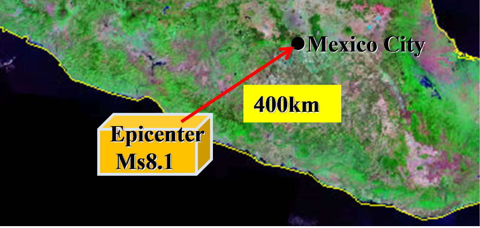
Figure 1. Epicenter of the 1985 Mexican earthquake.
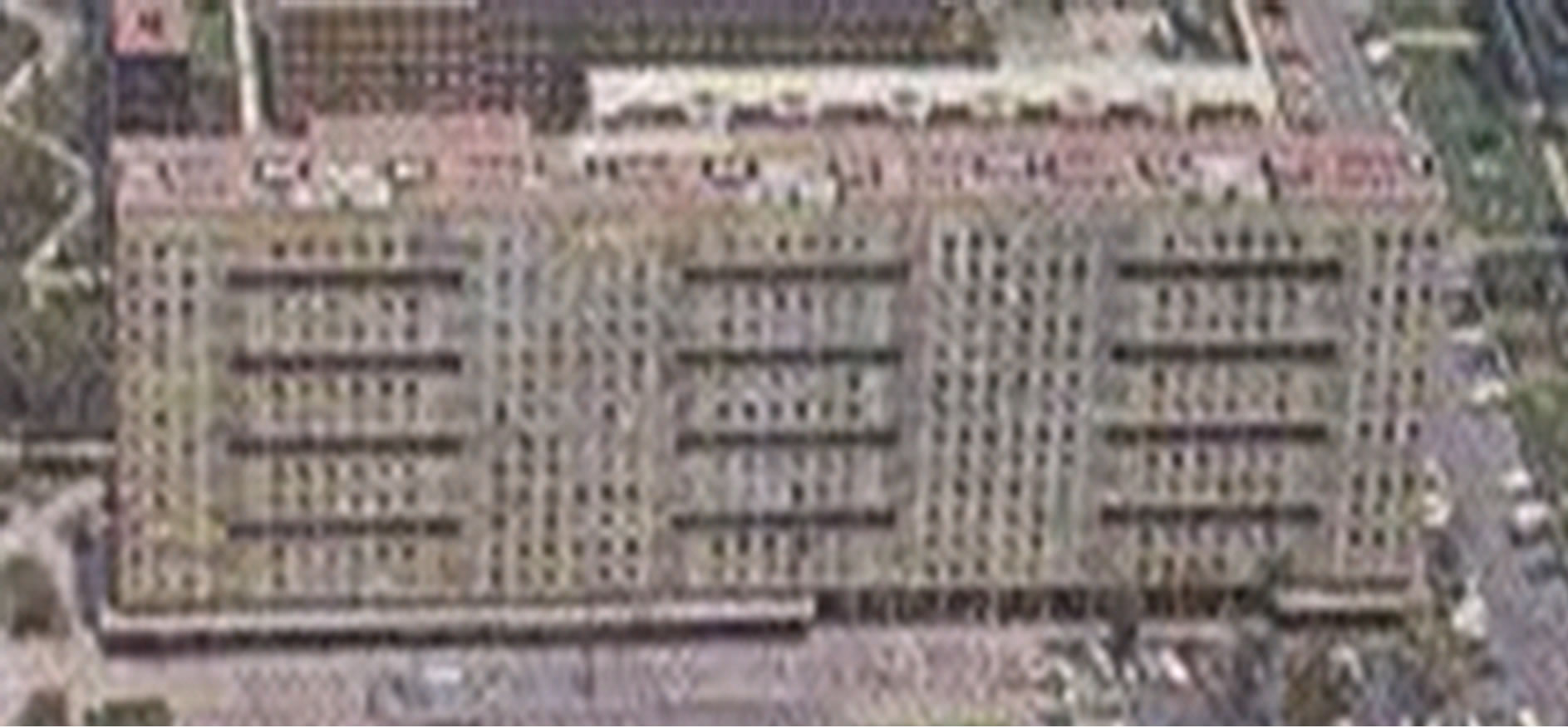
Figure 2. The Nuevo Leon buildings before the earthquake.
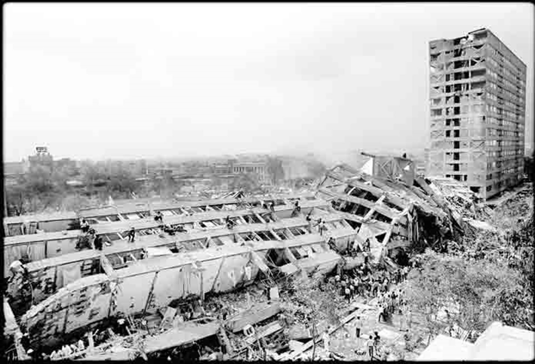
Figure 3. Collapse of the Nuevo Leon buildings (south building at the far side, picture by Marco Antonio Cruz).
approximately 0.5 Hz [3]. Therefore, nearly all of the 14-story buildings in the district, which had natural periods of approximately 2 s, were destroyed during the earthquake, as shown in Figure 4.
We investigated the seismic pounding phenomena due to the long-period ground motion by conducting analyses on a simulated model of Nuevo Leon buildings and two neighboring framed structures with different heights. We used a finite element code based on the adaptively shifted integration (ASI)-Gauss technique [4], which provides higher computational efficiency than the conventional code for this type of problem, and enables us to address dynamic behavior with strong nonlinearities, including phenomena such as member fracture and elemental contact. Contact release and re-contact algorithms are developed and implemented in the code to understand the complex behaviors of structural members during the seismic pounding and collapse sequence. In the analysis of the Nuevo Leon buildings, we set the natural period of one building to be 25% longer than those of the other buildings, as a difference in natural periods was observed in similar buildings based on the damage caused by previous earthquakes.
2. NUMERICAL METHODS
The general concept of the ASI-Gauss technique compared with the earlier version of the technique, the ASI
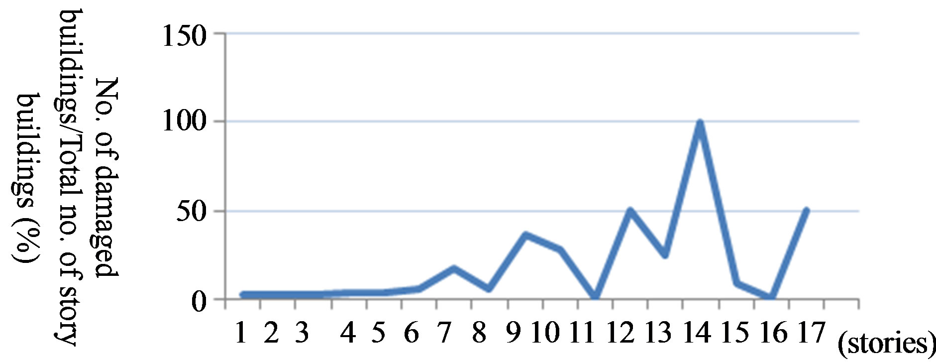
Figure 4. Ratio of the damaged buildings vs. story no. of buildings in the 1985 Mexican earthquake.
technique [5], is explained in this section. In addition, the algorithms considering member fracture, elemental contact, and incremental equation of motion for excitation at fixed points are described.
2.1. ASI-Gauss Technique
Figure 5 shows a linear Timoshenko beam element and its physical equivalence to the rigid bodies-spring model (RBSM). As shown in the figure, the relationship between the location of the numerical integration point and the stress evaluation point where a plastic hinge is formed is expressed as [6]
 (1)
(1)
where s is the location of the numerical integration point, and r is the location where the stresses and strains are actually evaluated. We refer to r as the stress evaluation point later in this report. The quantities for s and r are non-dimensional and take values between –1 and 1.
In both the ASI and ASI-Gauss techniques, the numerical integration point is shifted adaptively, when a fully plastic section is formed within an element, to create a plastic hinge at exactly that section. When the plastic hinge is determined to be unloaded, the corresponding numerical integration point is shifted back to its normal position. Here, the normal position is where the numerical integration point is placed when the element acts elastically. By doing so, the plastic behavior of the element is simulated appropriately, and the converged solution is achieved with only a small number of elements per member. However, in the ASI technique, the numerical integration point is placed at the midpoint of the linear Timoshenko beam element, which is considered to be optimal for one-point integration, where the entire region of the element behaves elastically. When the number of elements per member is small, solutions in the elastic range are not accurate enough because the onepoint integration is only used to evaluate the low-order displacement function of the beam element.
The main difference between the ASI and ASI-Gauss techniques lies in the normal position of the numerical integration point. In the ASI-Gauss technique, two consecutive elements forming a member are considered to
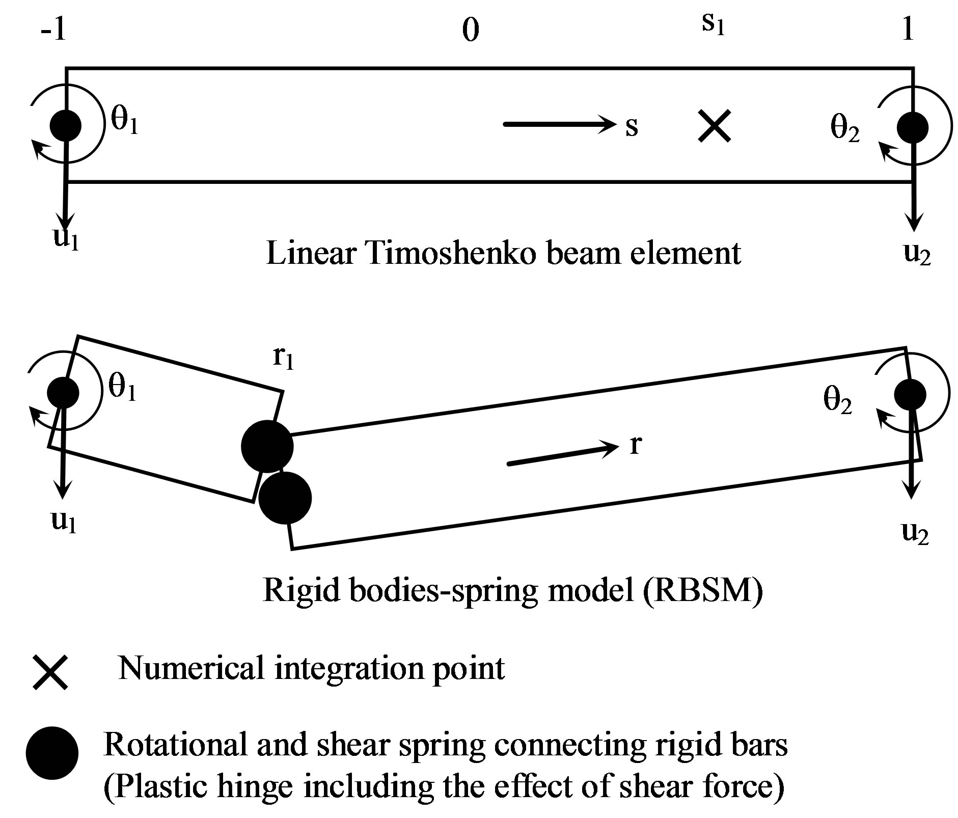
Figure 5. Linear Timoshenko beam element and its physical equivalent.
be a subset, and the numerical integration points of an elastically deformed member are placed such that the stress evaluation points coincide with the Gaussian integration points of the member. This means that the stresses and strains are evaluated at the Gaussian integration points of elastically deformed members. The Gaussian integration points are optimal for two-point integration, and the accuracy of bending deformation is mathematically guaranteed [7]. This way, the ASI-Gauss technique takes advantage of two-point integration while using one-point integration in the actual calculations.
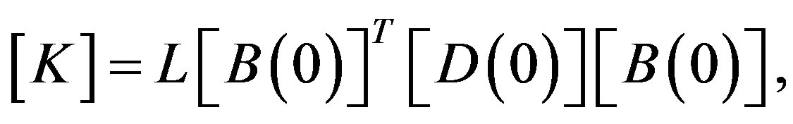
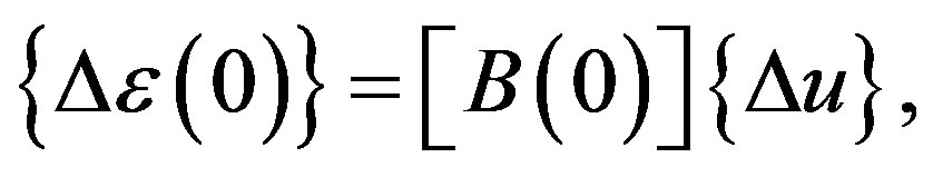
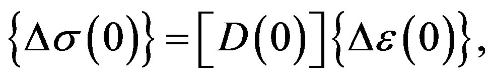
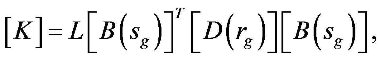
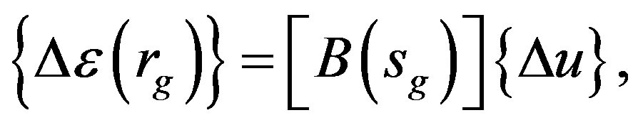
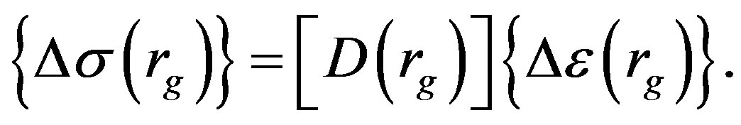
Figure 6 shows the locations of the numerical integrations points of elastically deformed elements in the ASI and ASI-Gauss techniques. The elemental stiffness matrix, the generalized strain and the sectional force increment vectors in the elastic range are given for the ASI and the ASI-Gauss techniques by Eqs.2 and 3, respectively.
 (2a)
(2a)
 (2b)
(2b)
 (2c)
(2c)
 (3a)
(3a)
 (3b)
(3b)
 (3c)
(3c)
here,  and
and  are the dimensionless coordinates in each element that have a value of
  and
and , respectively.
 ,
,  and
and  are the generalized strain increment vector, generalized stress (sectional force) increment vector and nodal displacement increment vector, respectively. [B] is the generalized strain-nodal displacement matrix, [D] is the stress-strain matrix, and L is the length of the element.
The plastic potential used in this study is expressed by
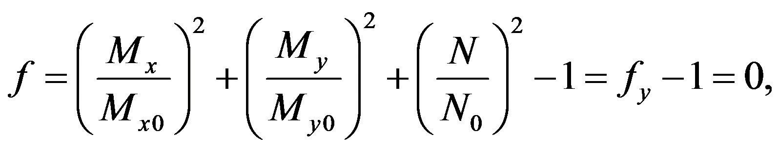 (4)
(4)
where 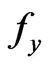 is the yield function, and
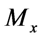 ,
, 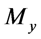 and
and  are the bending moments around the x-axis, the y-axis and the axial force, respectively. The terms with the subscript 0 are values that result in a fully plastic section in an element if they act on the cross section independently. The effect of torsion and shear force is neglected in the yield function.
2.2. Member Fracture and Contact Algorithm
A plastic hinge is likely to occur before it develops into a member fracture, and the plastic hinge is expressed by shifting the numerical integration point to the opposite end of the fully-plastic section. Accordingly, the numerical integration point of the adjacent element forming the same member is shifted back to its midpoint, where it is appropriate for one-point integration. Figure 7 shows the location of numerical integration points for each stage in the ASI-Gauss technique.
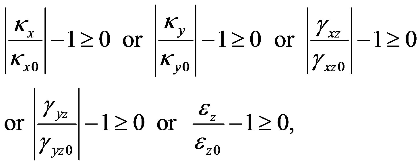
In this study, member fracture is determined by the curvatures, shear strains and axial tensile strain that oc-
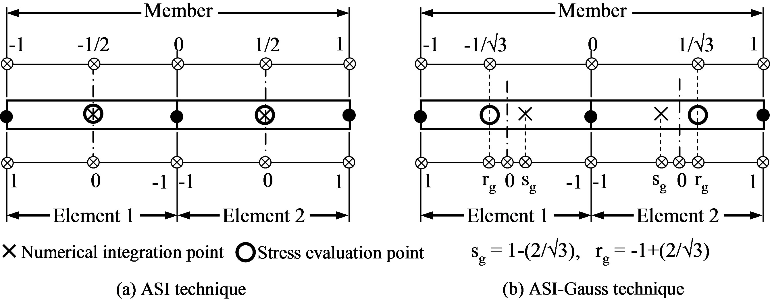
Figure 6. Locations of the numerical integration and stress evaluation points in the elastic range.
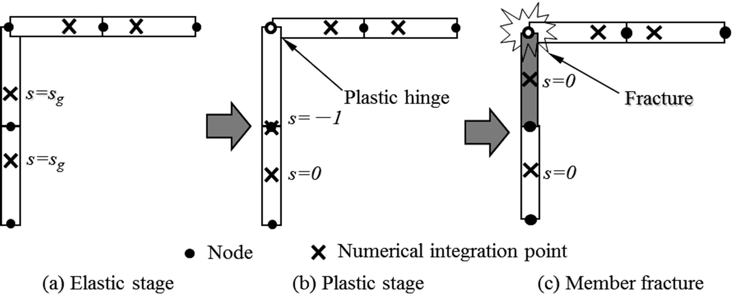
Figure 7. Locations of numerical integration points for each stage of the ASI-Gauss technique.
curred in the elements, as shown in the following equation.
 (5)
(5)
where  and
and ,
,  and
and ,
,  , and
, and ,
,  ,
,  ,
,  and
and  are the curvatures around the xand y-axes, the shear strains for the xand y-axes, the axial tensile strain and the critical values for these strains, respectively. The critical values were fixed using information from actual experimental data [8]. Contact determination is found by examining the geometrical locations of the elements, and once two elements are determined to be in contact, they are bound with four gap elements between the nodes [4]. The sectional forces are delivered through these gap elements to the connecting elements. To express contact release, the gap elements are automatically eliminated when the mean value of the deformation of gap elements is reduced to a specified ratio.
2.3. Incremental Equation of Motion
The dynamic equilibrium equation at time step t = t can be formulated as
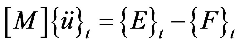 , (6)
, (6)
where ,
,  ,
,  and
and  are the mass matrix, acceleration vector, nodal external force vector and internal force vector at time step t = t, respectively.
The following equation is substituted into Eq.6 at t = t + 1 in the implicit code:
 (7)
(7)
Then, the following incremental stiffness equation is evaluated:
 (8)
(8)
where  is a stiffness matrix at time step t = t. By neglecting residual forces, an implicit code is obtained by evaluating the following incremental equation of motion:
 (9)
(9)
Consequently, the incremental equation of motion for a structure under excitation at fixed points, which are used in this report, yields the following:
 (10)
(10)
The subscript 1 indicates the coupled terms between the free nodes, 2 indicates the coupled terms between the free nodes and the fixed nodes, and b indicates the components at the fixed nodes. Vectors  and
and  are the nodal acceleration increment and the nodal displacement increment, respectively.
Under the assumption that the displacements at the free nodes are estimated by adding quasi-static displacement increments  and dynamic displacement increments
 , the displacements at the free nodes are given as
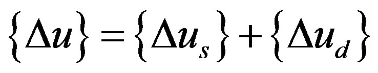 . (11)
 is evaluated, by neglecting inertia force, as follows:
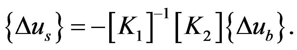 (12)
(12)
Substituting Eqs.11 and 12 into Eq.10, the following equation is obtained:
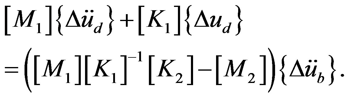 (13)
(13)
In this method, the equivalent forces are calculated by substituting nodal acceleration increments at the fixed points into the right side of the above equation.
3. SEISMIC POUNDING ANALYSIS OF NEIGHBORING BUILDINGS
A seismic pounding analysis is performed, using the numerical code shown above, on neighboring buildings to investigate the effects of collisions between them during a long-period ground motion.
3.1. Seismic Pounding Analysis of Neighboring Framed Structures with Different Heights
As shown in Figure 8, simple numerical models of two neighboring framed structures with different heights are constructed to investigate the seismic pounding behavior. One of the framed structures is 12-stories high, and the other is 7-stories high. The distance between the two models is 30 cm. Each story is 3.46 m high, with a span length of 6.3 m and a depth of 12.4 m. The sectional properties and the material properties of the models are shown in Tables 1 and 2, respectively. The floor loads are set to 4.5 kN/m2. The SCT seismic wave of the 1985 Mexican earthquake, as shown in Figure 9, is used for the input ground motion. The time increment for the analysis is 1 ms, and the total number of steps is 183,501. The critical curvatures for fracture are set to 3.333 × 10⁻⁴, the critical shear strains to 2.600 × 10⁻³ and the critical axial tensile strain to 0.17.
No impact occurred between the two structures throughout the analysis when the buildings were both 12-stories high. On the other hand, the models collided during the ground motion when one building was 7-stories high, and as shown in Figure 10, both eventually collapsed. The colors represent the distribution of the yield function values fy. This result shows that the distances between neighboring buildings are crucial and that the distances must be sufficiently secured, particularly if the natural periods of the buildings are different.
3.2. Seismic Pounding Analysis of Nuevo Leon Buildings
As shown in Figure 11, we constructed a simulated
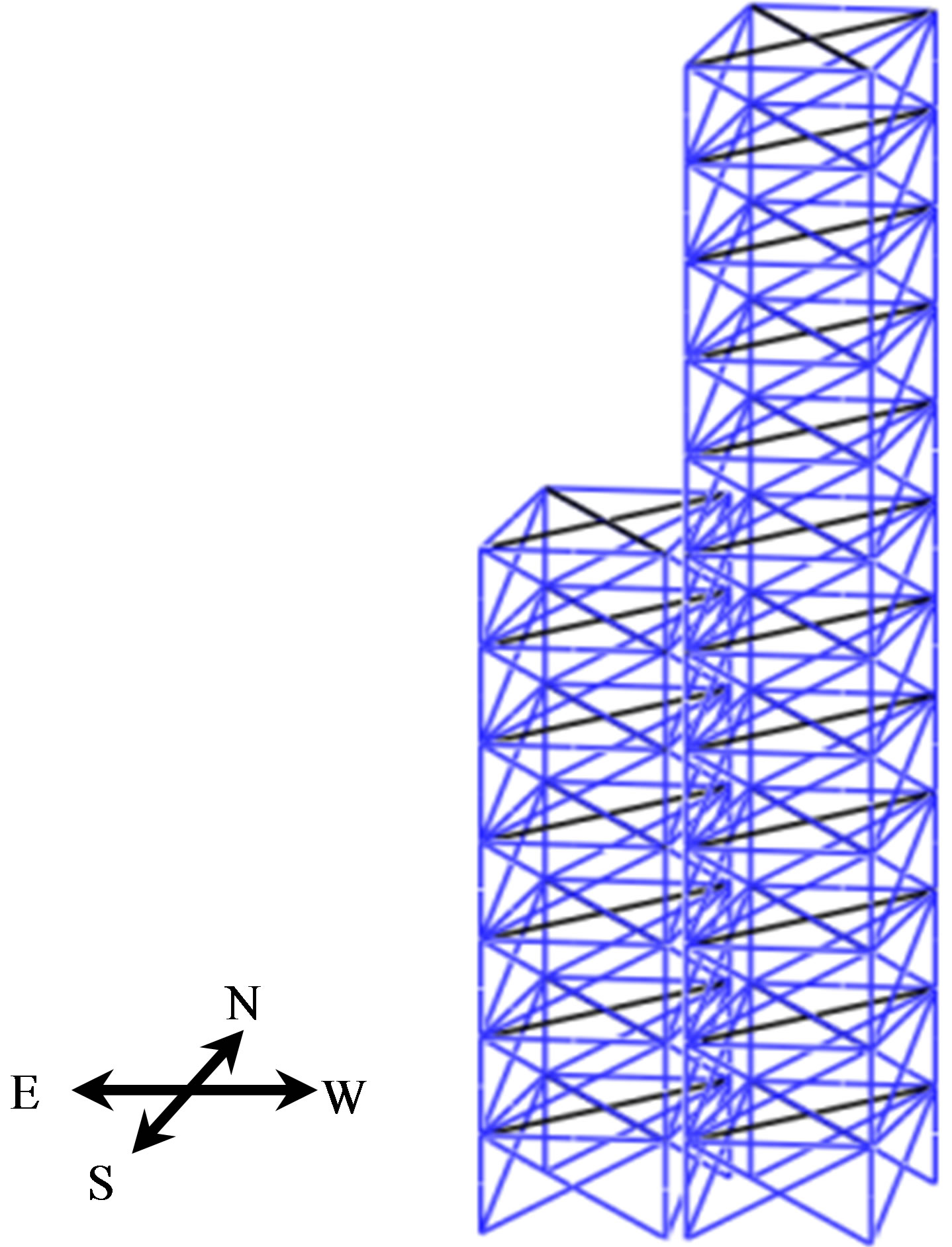
Figure 8. Numerical models of the two neighboring framed structures.

Table 1. Sectional properties of the structural members.
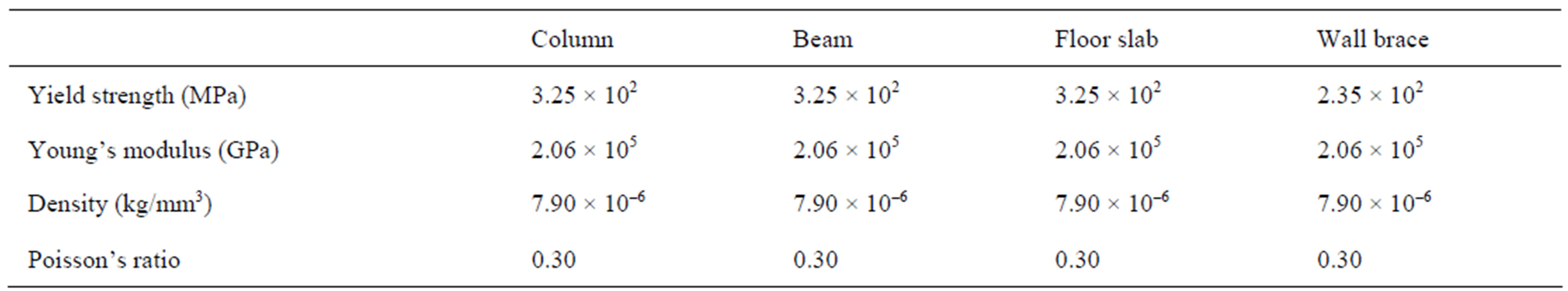
Table 2. Material properties of the structural members.
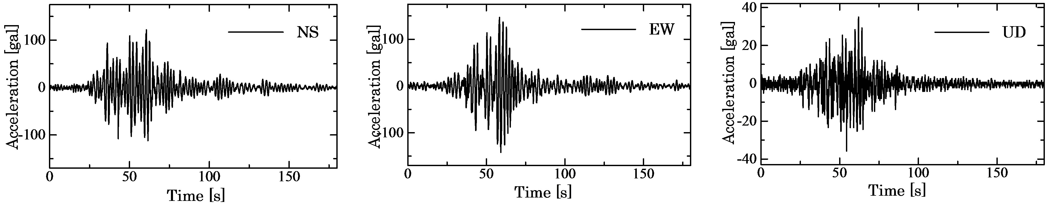
Figure 9. Input ground acceleration (SCT wave).
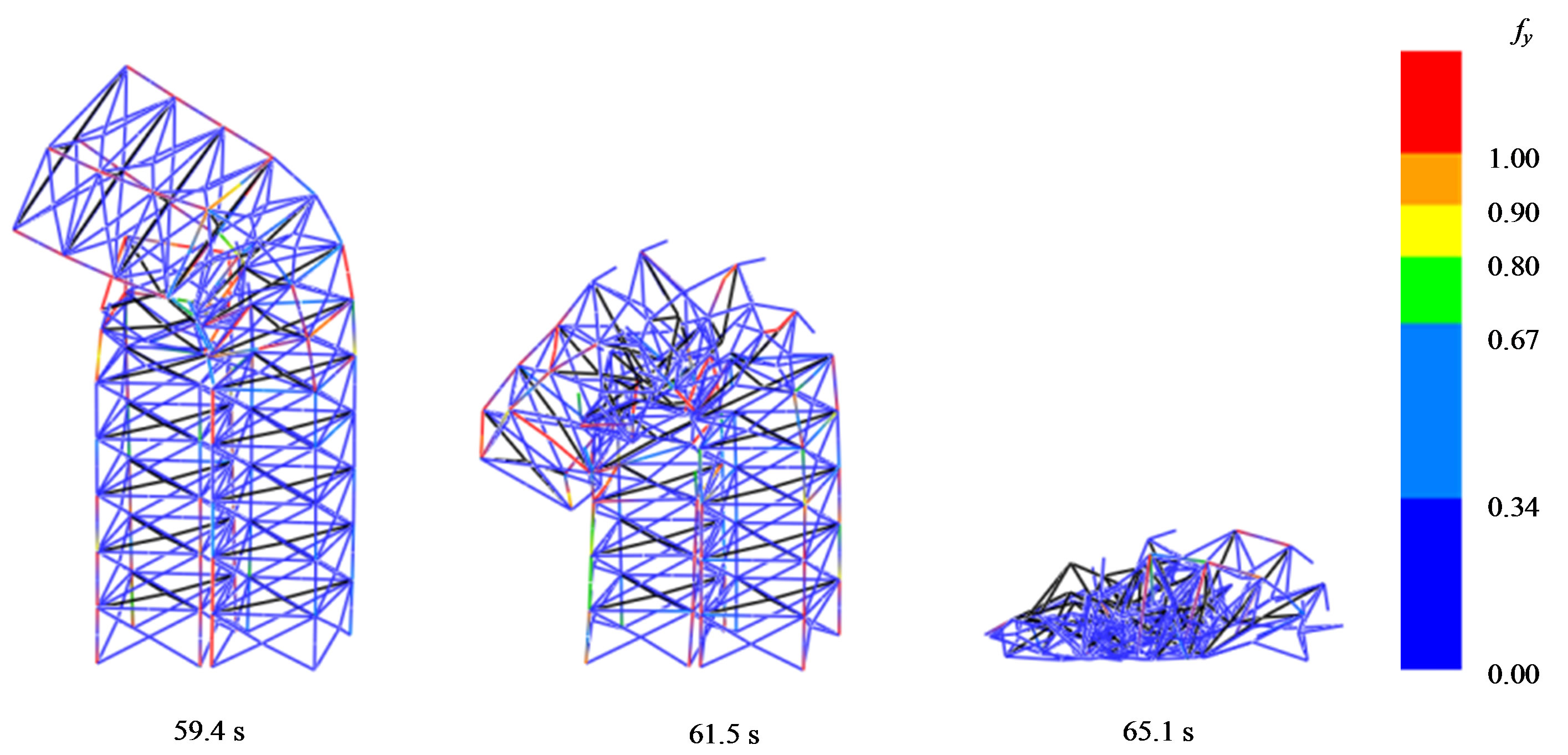
Figure 10. Collapse modes of the two neighboring framed structures.
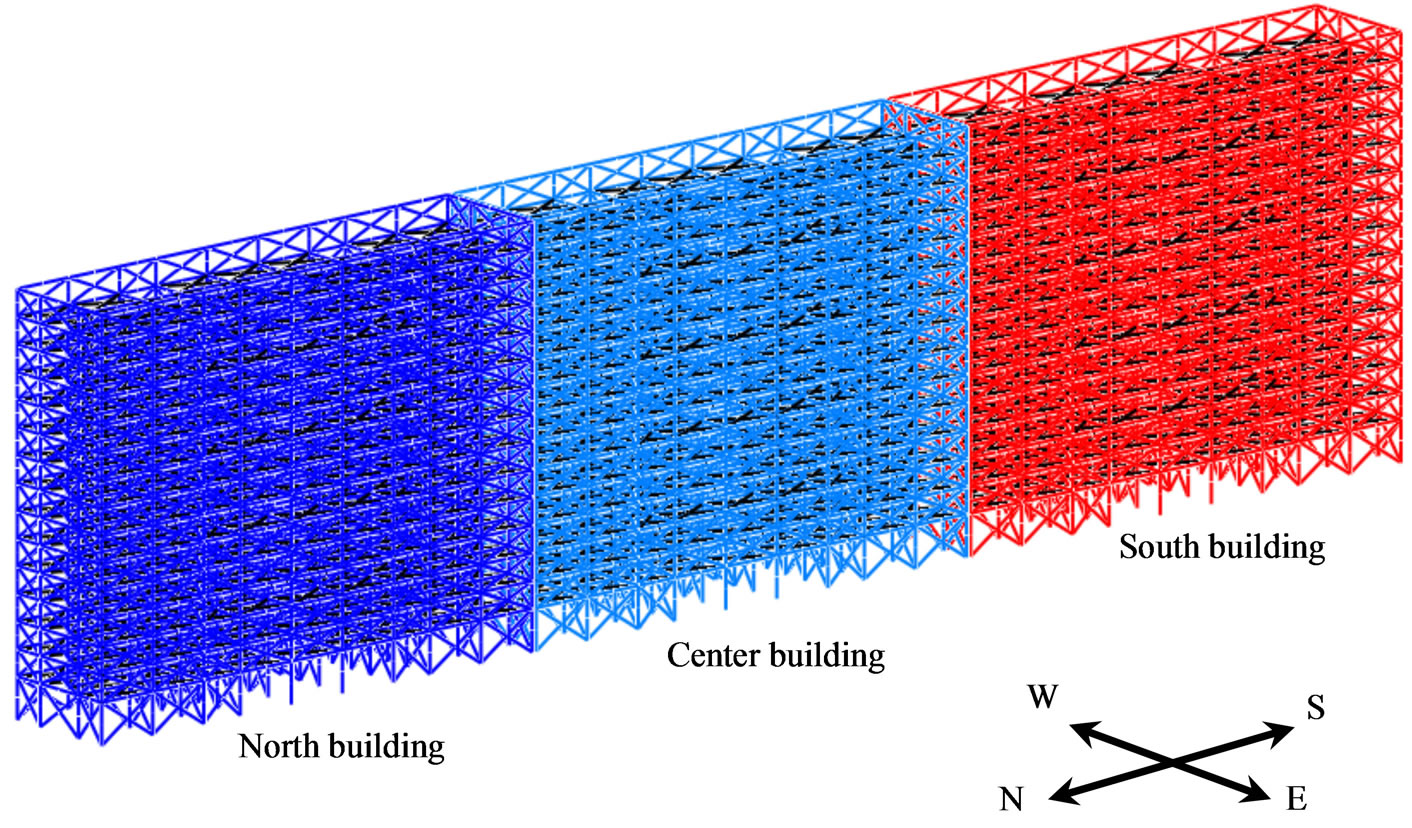
Figure 11. Numerical models of the three connected buildings.
model of the Nuevo Leon buildings with three similar 14-story buildings built consecutively with narrow gaps of 10 cm. The model is 42.02 m high and 12.4 m wide, with a total length of 160 m. By referring to the design guideline of Mexico in 1985, the base shear coefficient is set to 0.06, and the axial force ratio on the first floor is set approximately to 0.5. The dead load for each floor is set to 4.0 kN/m2, and the damping ratio is set to 5%. The Nuevo Leon buildings were originally built with reinforced concrete (RC) members; however, the model constructed in this study is intentionally made with steel members to easily verify the influence of the structural parameters, such as member fracture strains. The critical curvatures for the fracture are set to 3.333 × 10⁻⁴, the critical shear strains to 3.380 × 10⁻⁴ and the critical axial tensile strain to 0.17. The critical shear strains used are lower than the strain values of the steel members to consider the characteristics of RC beams. The sectional properties of the structural members are shown in Table 3. The time increment is set to 1 ms, and the calculation is performed for 90,000 steps. The analysis takes approximately 4 days using a personal computer (CPU: 2.93 GHz Xeon).
As shown in Table 4, we set the natural period of the north building model to be 25% longer than the other periods by lowering the structural strengths of the columns. The difference of natural periods was observed in similar buildings built near the site (see Table 5), caused by the damage from previous earthquakes [1]. The EW, NS and UD components of the SCT seismic wave shown in Figure 9 are subjected to the fixed points on the ground floor. As mentioned earlier, the intensity period of the seismic wave was approximately 2 s because of the reclaimed soft soil of Mexico Valley. According to the numerical results in Figure 12, the collision of the buildings may be a result of the difference in the natural periods between neighboring buildings. As shown in Figure 13, a collision first occurs between the north and

Table 3. Sectional properties of the structural members.
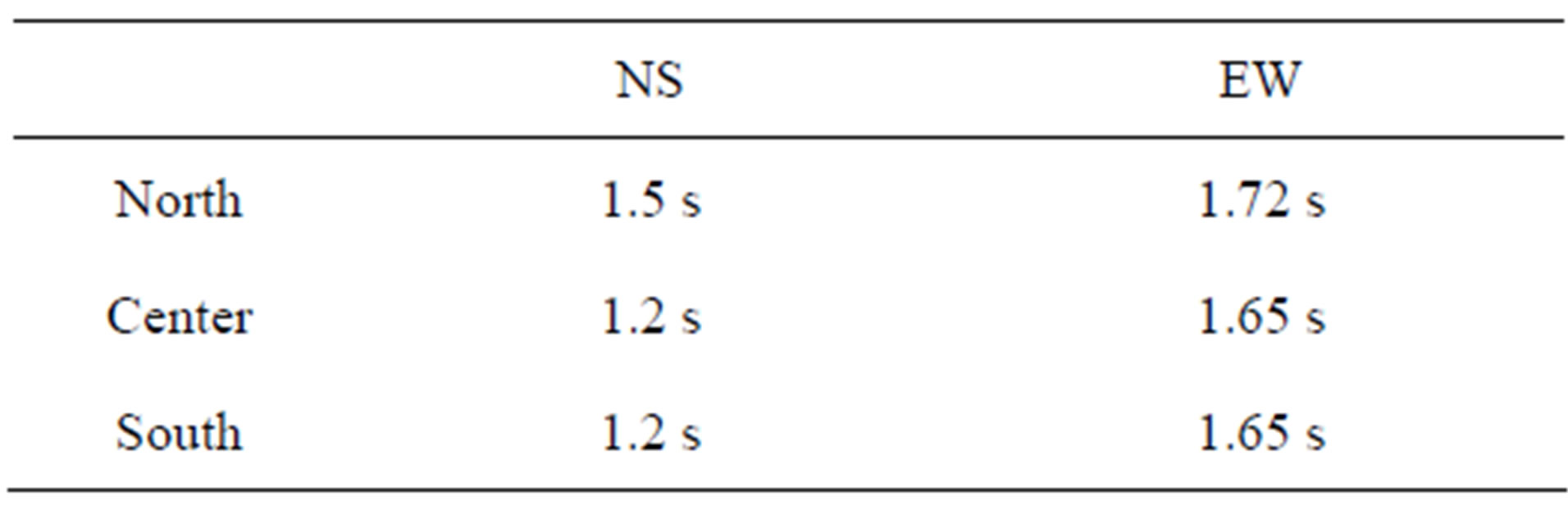
Table 4. Natural period of each building model.
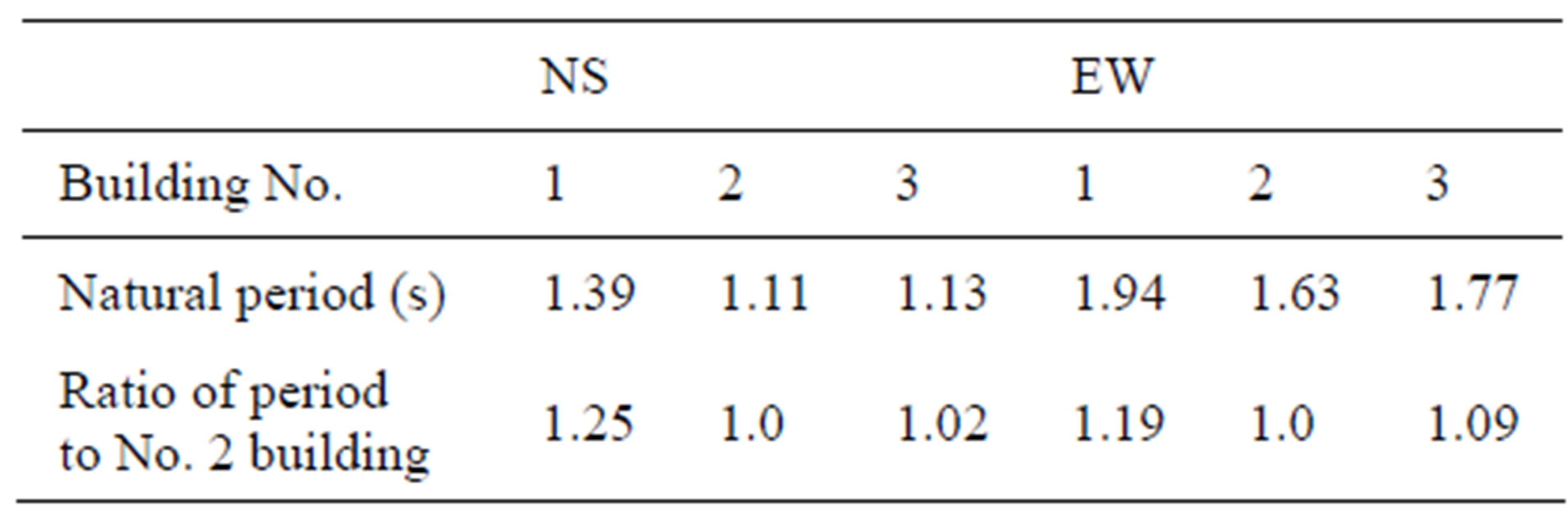
Table 5. Natural period of Chihuanua, a similar building.
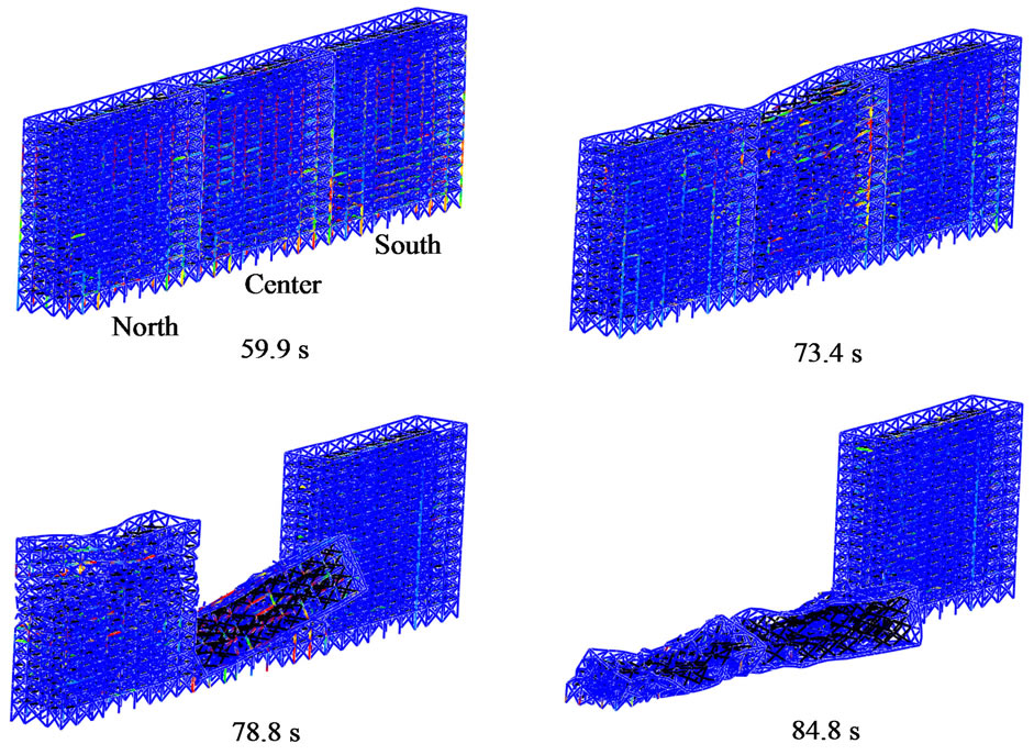
Figure 12. The collapse behaviors of the simulated model of the Nuevo Leon buildings under long-period ground motion.
center buildings due to the difference of the natural periods, and the plastic region spreads through the beams and columns. Then the columns near the impact point occasionally lose their structural strengths resulting from the continuous pounding sequence. The collapse of the center building is initiated at the ceiling of the 9th floor because of the continuous collisions from both sides, which begins approximately 70 s from the start of seismic activity. Although the north building collapses a few seconds after the center, the south building withstands the collisions and does not collapse as shown in Figure 12.
4. CONCLUSION
The numerical results shown in this report clarify the
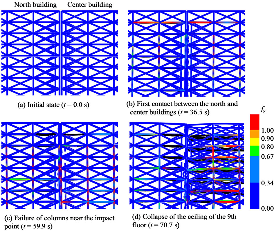
Figure 13. The impact and collapse initiation behaviors of the north and center buildings.
possibility that long-period ground motion may cause extra damage in high-rise buildings due to inter-building collisions, if the distances between them are not sufficiently secured. Extra caution may be needed if the natural periods of the neighboring buildings are different, which can easily occur, for example, if their heights are different.
5. ACKNOWLEDGEMENTS
The authors would like to express their appreciation for the contributions of these former students of the University of Tsukuba: Tetsuya Hisanaga, Takuya Katsu, Le Thi Thai Thanh and Yuta Arakaki.
REFERENCES
- Ciudad de Mexico (1986) Programa de reconstruccionNonoalco/Tlatelolco, Tercerareunion de la Comision Tecnica Asesora. The Third Meeting of the Technical Commission Advises, Ciudad de Mexico.
- Universidad Nacional Autonoma de Mexico (1985) The earthquake of September 19th, 1985. Inform and preliminary evaluation. Universidad Nacional Autonoma de Mexico.
- Celebi, M., Pince, J., Dietel, C., Onate, M. and Chavez, G. (1987) The culprit in Mexico City—Amplification of motions. Earthquake Spectra, 3, 315-328. doi:10.1193/1.1585431
- Lynn, K.M. and Isobe, D. (2007) Finite element code for impact collapse problems of framed structures. International Journal for Numerical Methods in Engineering, 69, 2538-2563.doi:10.1002/nme.1858
- Toi, Y. and Isobe, D. (1993) Adaptively shifted integration technique for finite element collapse analysis of framed structures. International Journal for Numerical Methods in Engineering, 36, 2323-2339. doi:10.1002/nme.1620361402
- Toi, Y. (1991) Shifted integration technique in one-dimensional plastic collapse analysis using linear and cubic finite elements. International Journal for Numerical Methods in Engineering, 31, 1537-1552. doi:10.1002/nme.1620310807
- Press, W.H., Teukolsky, S.A., Vetterling, W.T. and Flannery, B.P. (1992) Numerical recipes in FORTRAN: The art of scientific computing. Cambridge University Press, New York.
- Hirashima, T., Hamada, N., Ozaki, F., Ave, T. and Uesugi, H. (2007) Experimental study on shear deformation behavior of high strength bolts at elevated temperature. Journal of Structural and Construction Engineering, 621, 175-180.