Natural Science
Vol.4 No.1(2012), Article ID:16594,5 pages DOI:10.4236/ns.2012.41012
A simple piecewise cubic spline method for approximation of highly nonlinear data
![]()
Civil Engineering Department, Faculty of Technical and Engineering, Yasouj University, Yasouj, Iran; mahdi@mail.yu.ac.ir
Received 14 September 2011; revised 20 October 2011; accepted 30 October 2011
Keywords: Simulation; Data analysis; Approximation; Cubic Spline; Optimization; Curve Fitting
ABSTRACT
Approximation methods are used in the analysis and prediction of data, especially laboratory data, in engineering projects. These methods are usually linear and are obtained by least-square-error approaches. There are many problems in which linear models cannot be applied. Because of that there are logarithmic, exponential and polynomial curve-fitting models. These nonlinear models have a limited application in engineering problems. The variation of most data is such that the nonlinearity cannot be approximated by the above approaches. These methods are also not applicable when there is a large amount of data. For these reasons, a method of piecewise cubic spline approximation has been developed. The model presented here is capable of following the local nonuniformity of data in order to obtain a good fit of a curve to the data. There is C1 continuity at the limits of the piecewise elements. The model is tested and examined with four problems here. The results show that the model can approximate highly nonlinear data efficiently.
1. INTRODUCTION
There are many cases in engineering activities in which one is confronted with laboratory or field data. Suppose there are n pairs of data values (xi, yi), where these values are obtained from experimental, field or statistical analysis. The aim is to find a function f(x) that predicts acceptable values for the dependent variable y with respect to the independent variable x. There are always some errors in the experimental analysis, and in the sensitivity and calibration of measuring instruments, and therefore the values of yi are not exact. Also, sometimes there exist multiple values for yi for each value of xi. In such situations, if the curve of f(x) passes between and near to the data points, it is more accurate and smoother than when it passes through all the points exactly. Thus, in those cases an approximate analysis is more suitable for predicting and assigning the y values. If the curve governing f(x) were instead to interpolate such data, it would have a sinusoidal or unsmoothed zigzag form that would not be acceptable and would not be usable for data analysis. Most of the publications about this subject are related mainly to linear or simple nonlinear models [1-4]. Some more advanced methods in this field are based on B-spline and Bézier curves [5-7]. These methods are used most for computer graphic. Because of the waviness and the sinusoidal forms of their curves, they are not applicable to engineering problems.
2. FORMULATION
Formulation of Problem
If the variation of the data follows a simple nonlinear curve, a single cubic spline function can be applied in the form of the following equation:
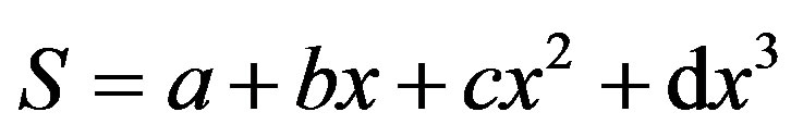 . (1)
. (1)
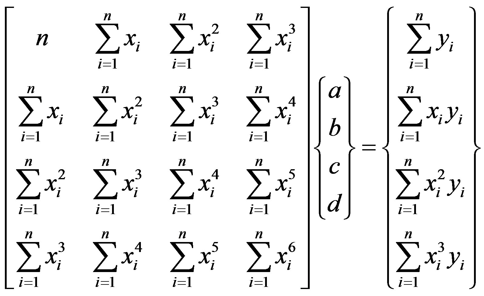
The parameters a, b, c and d are obtained by the method of least-square-error approximation from the solution of the following system of equations:
 , (2)
, (2)
where n is the number of pairs of data values in the interval [a, b]. In the case of the nonuniform variation of data that occurs in most engineering problems, a single cubic spline curve cannot be applied. Instead, it is necessary to use piecewise cubic spline curves to approximate such data. Suppose the distribution of data is as in Figure 1, for example.
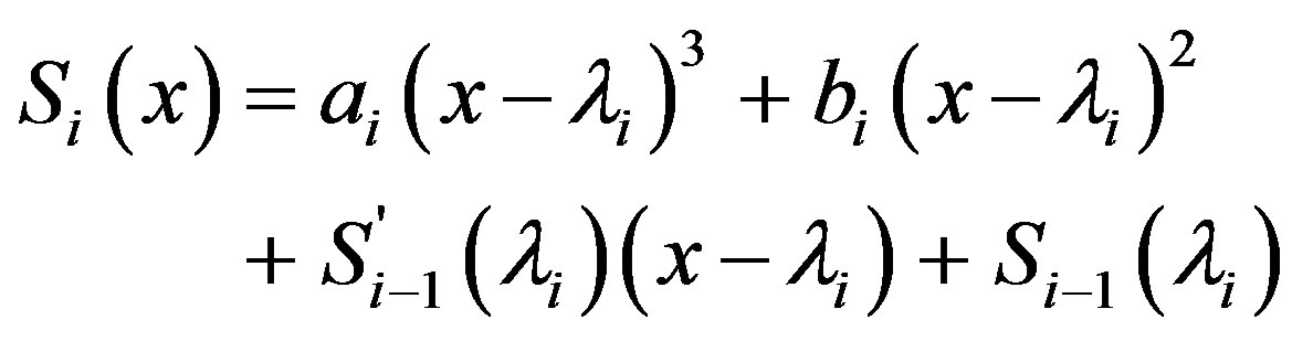
The domain of the problem is divided into n elements. The interval for the element i is [li, li+1]. The cubic spline equation for this element i is
 . (3)
. (3)
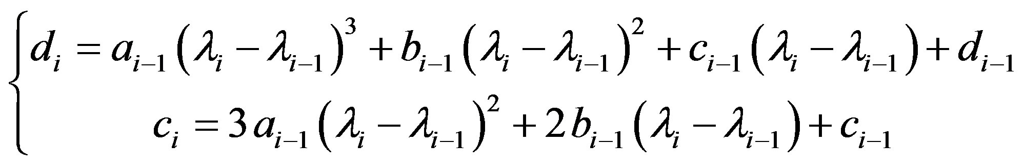
At the edges of each element, C1 continuity exists:
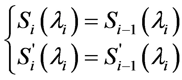 . (4)
. (4)
The parameters ,
,  ,
,  and
and  are obtained from Eqs.5-7 below, together with the continuity conditions of Eq.4, by minimization of the sum of squared errors (SSE):
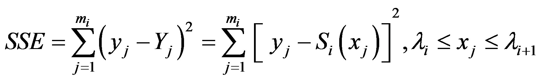 , (5)
, (5)
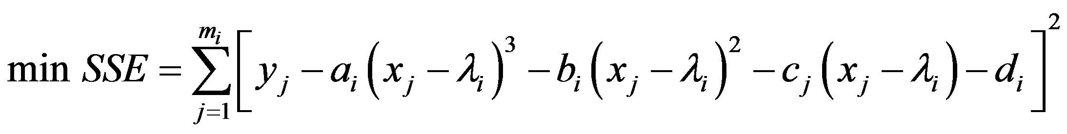 (6)
(6)
subject to the constraints,
 (7)
(7)
The minimization of Eq.6 by the use of Lagrange multipliers mi and ni is expressed as follows:
 (8)
(8)
To obtain the governing parameters, the derivatives of Eq.8 are calculated so that,
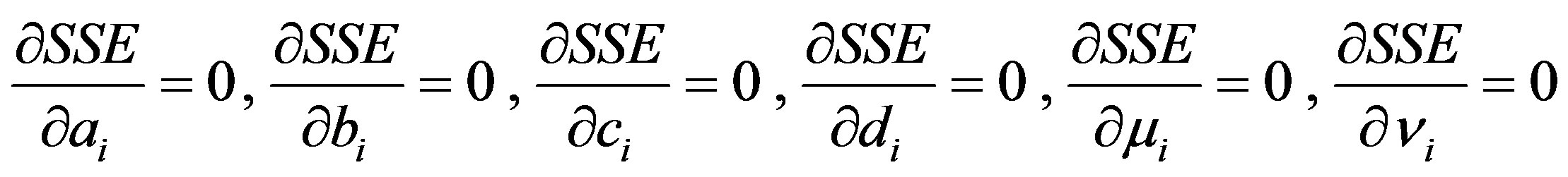 . (9)
. (9)
The above equations are transformed to a 6 6 linear system of equations for each element:
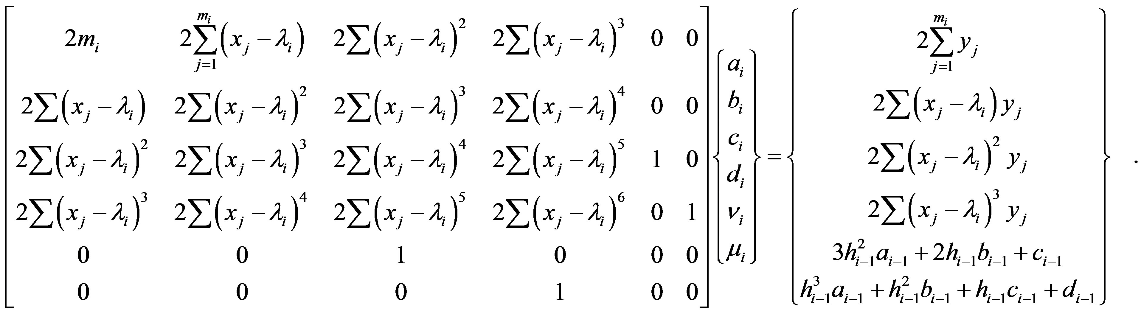 (10)
(10)
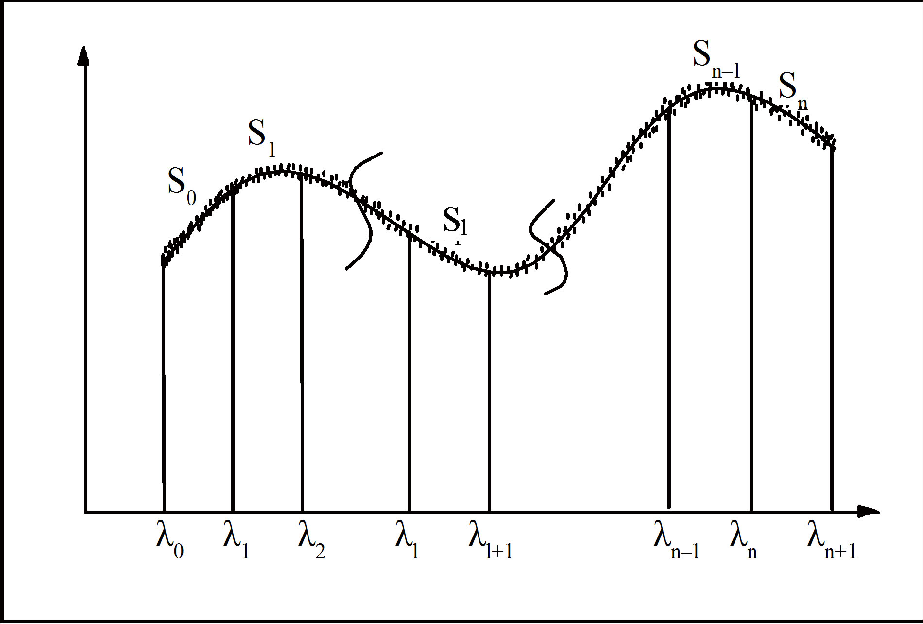
Figure 1. Behavior of a distribution of nonuniform data.
The linear system of Eq.10 is a local system, and all of these systems must be put together to make up a global linear system of equations with dimension 6n 6n. The parameters for each spline function are calculated by solving the global linear system. If there is a large number of data points, the dimension of the governing linear system of equations increases drastically and its solution becomes time-consuming. Therefore, in order to decrease the number of calculation operations, we can apply the following approach. If the continuity conditions of Eq.4 are inserted into Eq.3, the following equation results,
 (11)
(11)
The values of  and
and  in the above equation can be calculated numerically, taking account of the form of the variation of the data. Thus, the four parameters of Eq.11 are reduced to two. This decreases the number of related calculation operations by a large amount. Then, by optimizing the sum of squared errors, the parameters ai and bi can be obtained from the following equation:
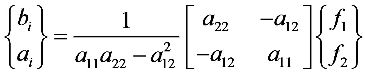 , (12)
in which
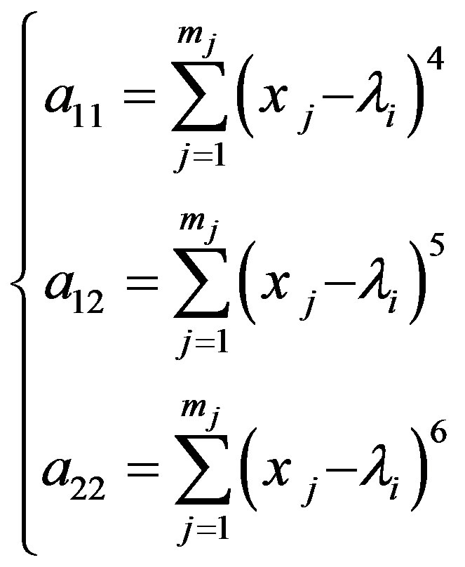 (13)
(13)
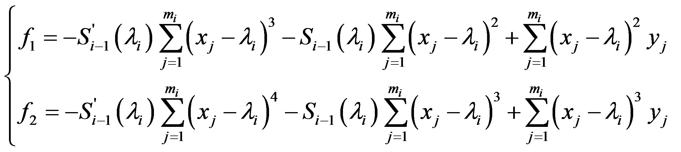
and Eq.14 (see the bottom of the page).
The boundary conditions for Eq.11 are  and
and . Four problems were selected for verification and examination of the model presented here.
3. PROBLEMS
3.1. Problem 1
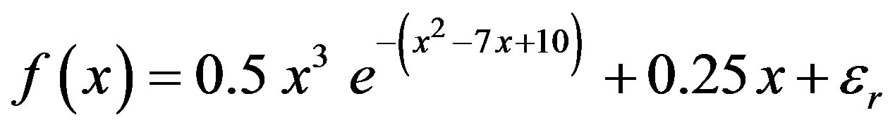
About 41 pairs of data values  were generated from the following equation,
 (14)
(14)
 , (15)
where  is a uniform random number between 0 and 1. For simplicity and to reduce the number of calculations, two cubic spline elements were used. Figure 2 illustrates the data distribution for the interval [1,5]. As can be seen, there is a good relationship between the piecewise cubic spline curves and the set of data. Therefore the model that we have developed can satisfactorily approximate this set of data.
3.2. Problem 2
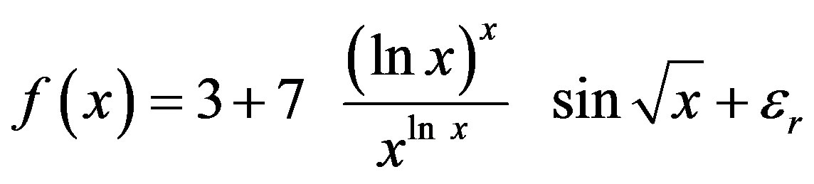
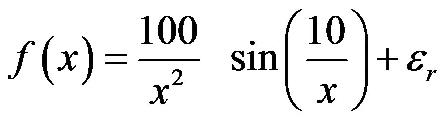
This example consisted of 81 pairs of data values on the interval [0, 8]. These were generated from the following equation:
 . (16)
Nonuniform elements were applied here because of the complexity and heterogeneity of the data distribution. The locations of the element boundaries are listed in Table 1. Figure 3 illustrates the data distribution and the calculated piecewise spline curve. As can be observed from the graph, there is a satisfactorily close relationship between the data and the curve.
3.3. Problem 3
For this problem, about 76 pairs of data values were generated from the following equation [8] on the interval [1,3] with nonuniform 
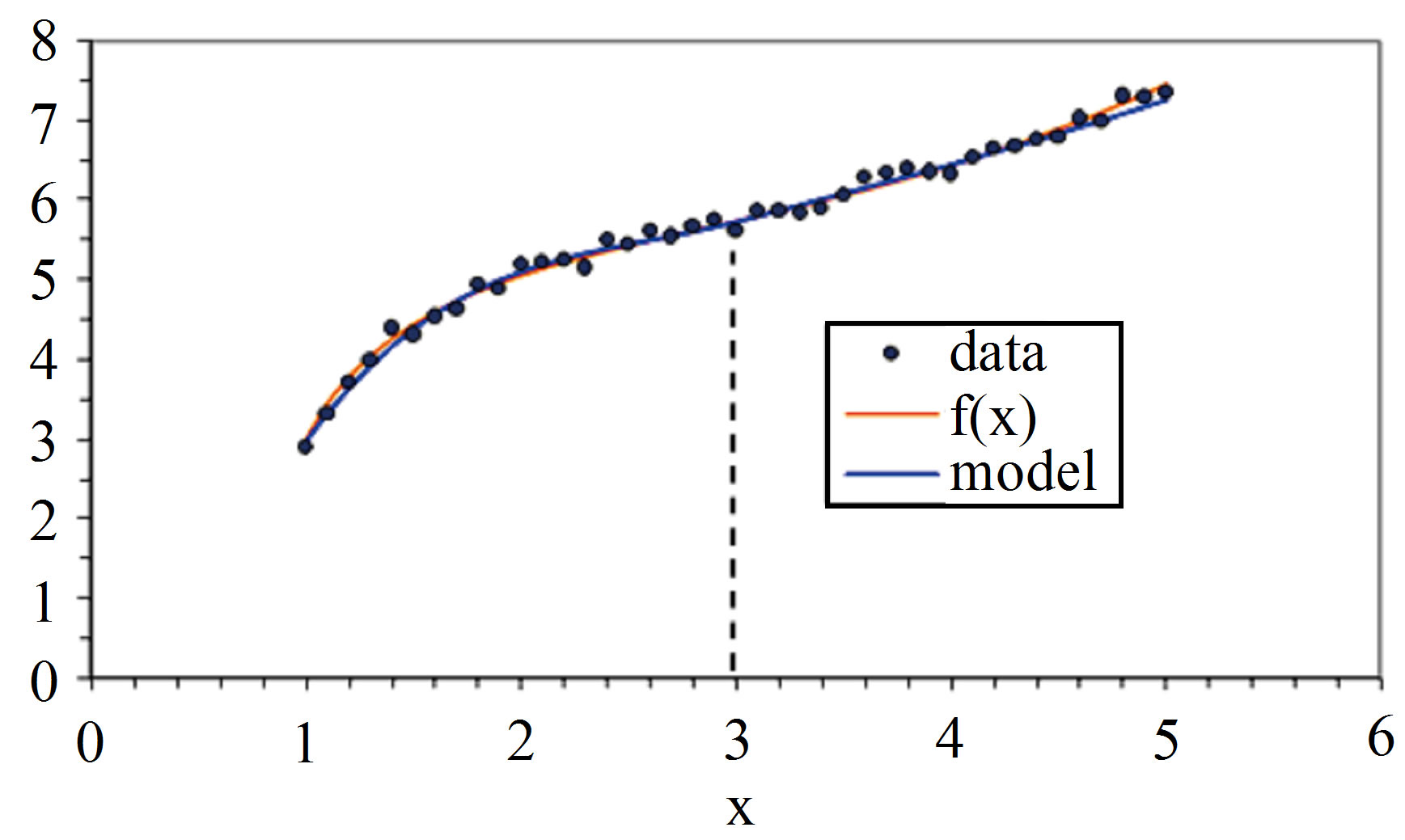
Figure 2. Comparison between spline curves and real data.
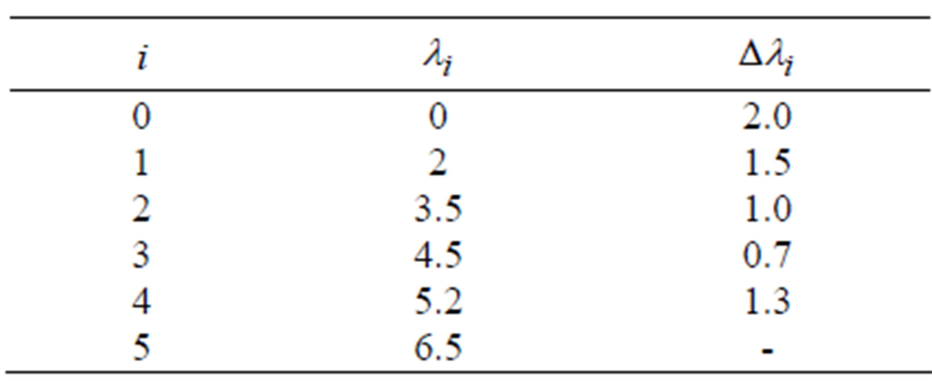
Table 1. Characteristics of the spline curve elements.
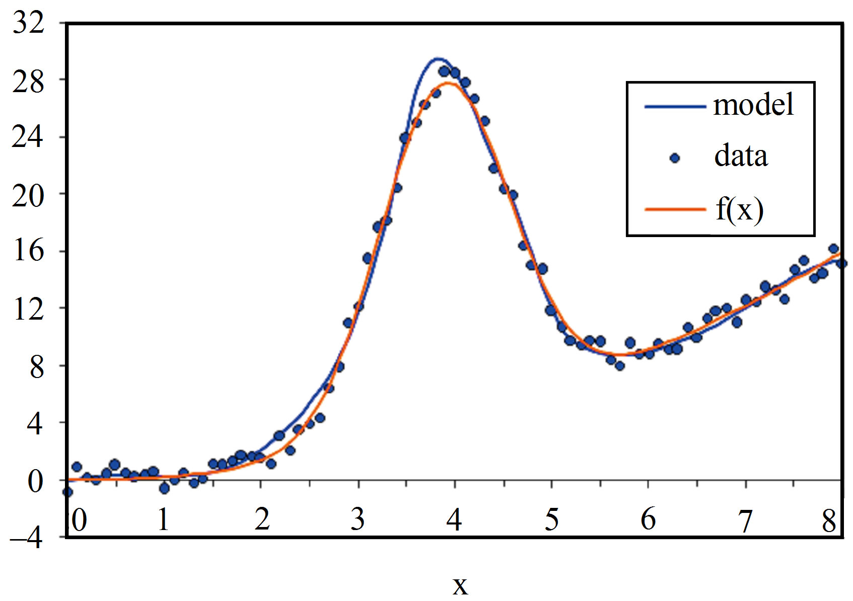
Figure 3. Comparison between real data and model.
 . (17)
The above equation is highly nonlinear and its variation is heterogeneous. A cubic spline curve consisting of eight pieces was developed for this example, based on the characteristics of the elements listed in Table 2. Figure 4 shows a comparison between the spline curve and the data for this test problem. The figure shows that there is a very close superimposition between the model and the governing data.
3.4. Problem 4
This problem is in the field of groundwater engineering. Theis solution for the nonequilibrium partial differential equation for unsteady radial flow from confined aquifer to pumping well is:
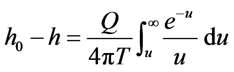 (18)
(18)
Thies approximated the above equation by the following series:
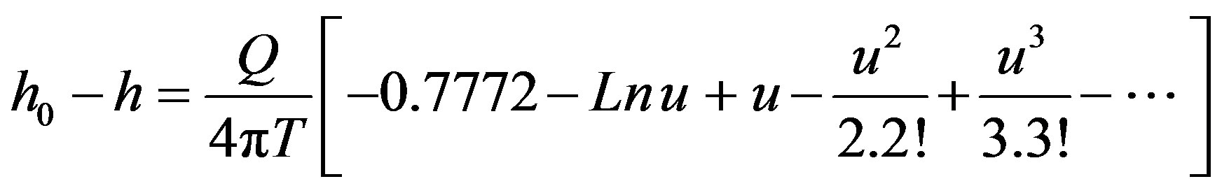 (19)
(19)
The value of brackets equals W(u) well function. The data for approximation have logarithm value of W(u) respect to logarithm value of u [9]. A cubic spline curve consisting of five pieces was developed for this problem, based on the characteristics of the elements listed in Table 3. Figure 5 illustrates the data distribution for the
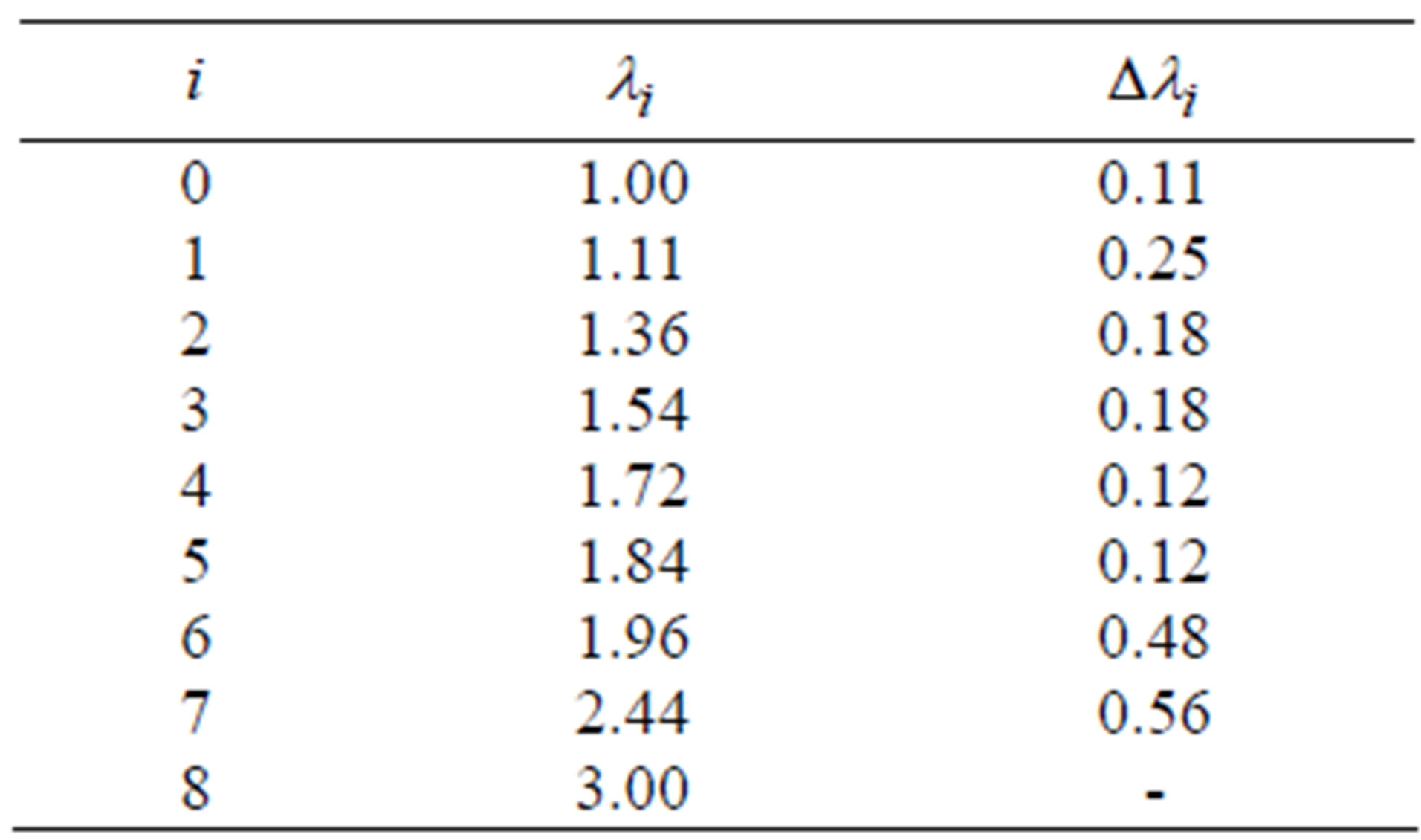
Table 2. Characteristics of the spline curve elements.
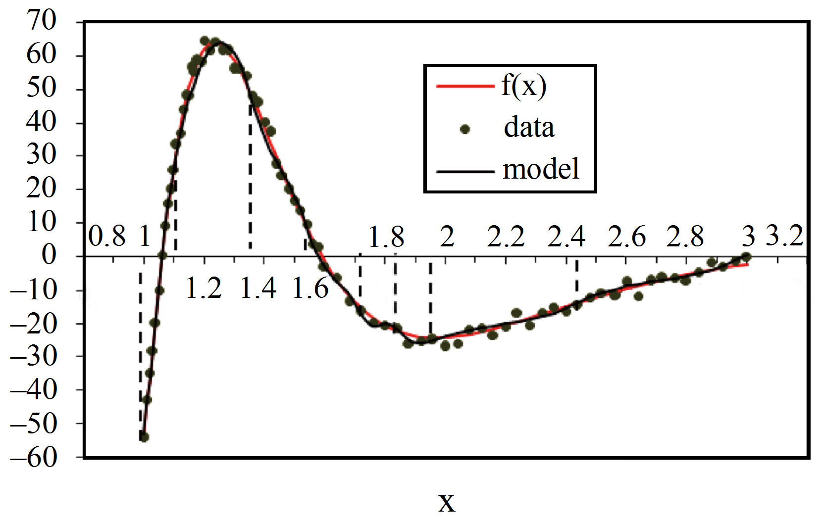
Figure 4. Comparison between real data and model.
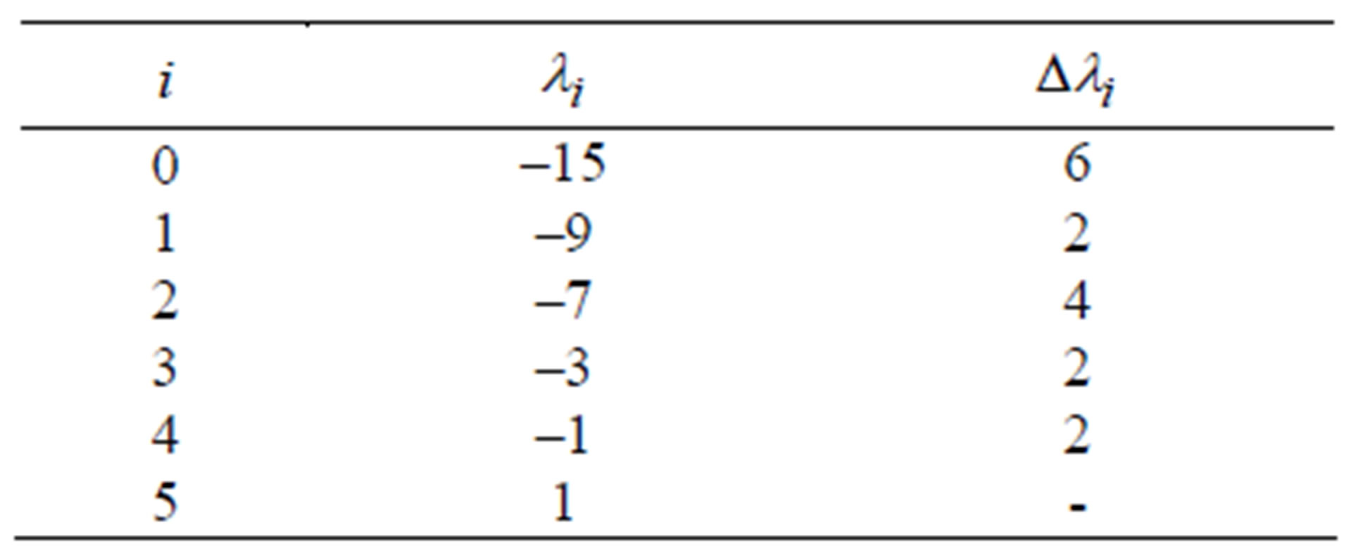
Table 3. Characteristics of the spline curve elements.
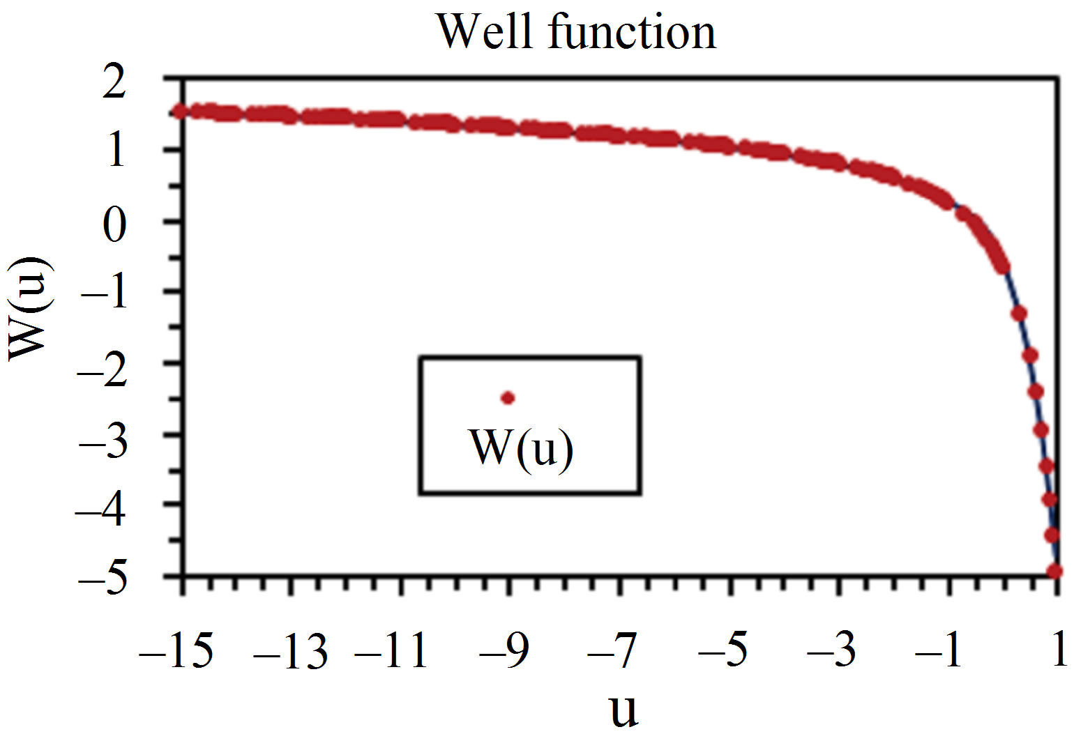
Figure 5. Comparison between real data and model.
interval [−15, 1]. According to the graph, there is an acceptable close relationship between the data and the cubic spline curve.
4. RESULTS AND CONCLUSIONS
The model presented above for the approximation of data with highly nonlinear variation can be applied efficiently to various engineering problems. Because the model’s formulation is straightforward and explicit, there is no need to establish and solve any linear system of equations. Therefore; the number of calculation operations related to the generation of piecewise cubic curves is noticeably less than that for other classical methods of approximation. I suggest that this formulation and model could be extended to two-dimensional approximation analysis. For this purpose, more attention must be paid to defining the formulation accurately, especially the satisfaction of the continuity conditions at the boundaries between elements or patches.
REFERENCES
- De Boor, C. (1978) A practical guide to splines. SpringerVerlag, Berlin, 472. doi:10.1007/978-1-4612-6333-3
- Conte, S.D. and De Boor, C. (1980) Elementary numerical analysis: An algorithm approach. 3rd Edition, McGrawHill, Auckland, 432.
- Lobo, N.A. (1995) Curve fitting using spline sections of different orders. Proceedings of the 1st International Mathematica Symposium, Southampton, 16-20 July, 267- 274.
- Zamani, M. (2009) Three simple spline methods for approximation and interpolation of data. Contemporary Engineering Sciences Journal, 2, 373-381.
- Lehmann, T.M., Gonner, C. and Spitzer, K. (2001) Bspline interpolation in medical image processing. IEEE Transactions on Medical Imaging, 20, 660-665. doi:10.1109/42.932749
- Salomon, D. (2006) Curves and surfaces for computer graphics. Springer, Northridge, 460.
- Zamani, M. (2009) An investigation of Bspline and Bezier methods for interpolation of data. Contemporary Engineering Sciences Journal, 2, 361-371.
- Burden, R.L. and Fairs, J.D. (1989) Numerical analysis. 4th Edition, PWS-Kent, Boston, 730.
- Todd, D.K. (1980) Groundwater hydrology. 2nd Edition, Wiley, New York, 535.