Received 22 October 2015; accepted 28 December 2015; published 31 December 2015

ABSTRACT

The spin-charge-family theory is a kind of the Kaluza-Klein theories, but with two kinds of the spin connection fields, which are the gauge fields of the two kinds of spins. The SO(13,1) representation of one kind of spins manifests in d = (3 + 1) all the properties of family members as assumed by the standard model; the second kind of spins explains the appearance of families. The gauge fields of the first kind, carrying the space index, manifest in d = (3 + 1) all the vector gauge fields assumed by the standard model. The gauge fields of both kinds of spins, which carry the space index (7, 8) gaining at the electroweak break nonzero vacuum expectation values, manifest in d = (3 + 1) as scalar fields with the properties of the Higgs scalar of the standard model with respect to the weak and the hyper charge (and, respectively), while they carry additional quantum numbers in adjoint representations, offering correspondingly the explanation for the scalar Higgs and the Yukawa couplings, predicting the fourth family and the existence of several scalar fields. The paper 1) explains why in this theory the gauge fields are with the scalar index doublets with respect to the weak and the hyper charge, while they are with respect to all the other charges in the adjoint representations; 2) demonstrates that the spin connection fields manifest as the Kaluza-Klein vector gauge fields, which arise from the vielbeins; and 3) explains the role of the vielbeins and of both kinds of the spin connection fields.

Keywords:

Unifying Theories, Beyond the Standard Model, Origin of Families, Origin of Mass Matrices of Leptons and Quarks, Properties of Scalar Fields, Origin and Properties of Gauge Bosons, Flavour Symmetry, Kaluza-Klein Theories

1. Introduction

The standard model assumed and the LHC confirmed the existence of the Higgs’s scalar―the only so far observed boson with the fractional charges. The question arises: where does the Higgs originate, why does it carry the “fermion” charges and where do the Yukawa couplings originate?

It is demonstrated in this paper how do the scalar fields with the weak and the hyper charge equal to and, respectively, appear from the simple starting action of the spin-charge-family theory. While the weak and

the hyper charge of the scalar gauge fields originate in the scalar index ¹, all the other charges of these scalar fields originate in the two kinds of the spin, carrying these additional charges in the adjoint representations. These scalars explain the appearance of families, of the Higgs scalar and the Yukawa couplings and their influence on the properties of the family members and on the families.

The relation between the vector gauge fields, when they are presented by the spin connections―this is the case in the spin-charge-family theory―and the vector gauge fields when they are expressed in terms of the vielbeins―which is usually used in the Kaluza-Klein theories―is discussed.

It was demonstrated in the paper [1] that all the scalars, that is all the gauge fields with the space index of the spin-charge-family theory, manifest in fractional charges with respect to the index s and the standard model charge groups: when carrying the space index they are doublets (originating in). When carrying the space index they are colour charge triplets (belonging to). Doublets explain the weak and the hyper charge; triplets offer a possible explanation for the matter-antimatter asymmetry of the ordinary matter in the universe and for the proton decay.

The spin-charge-family theory [2] -[12] offers the explanation for all the assumptions of the standard model: for the properties of each family member―quarks and leptons, left and right handed (right handed neutrinos are in this theory regular members of each family)―for the appearance of the families, for the existence of the gauge vector fields of the family member charges and for the scalar field and the Yukawa couplings. It is offering the explanation also for the existence of phenomena, which are not included in the standard model, like there is the dark matter [11] and the (ordinary) matter-antimatter asymmetry [1] .

The spin-charge-family theory predicts that there are at the low energy regime two decoupled groups of four families: The fourth [2] [4] [5] [10] to the already observed three families of quarks and leptons will be measured at the LHC [12] , LHC will measure also some of the scalar fields (manifesting as the Higgs and the Yukawa couplings [4] ). The lowest of the upper four families constitutes the dark matter [11] .

In Subsection 1.1 a short introduction of the spin-charge-family theory is made: the simple starting action of the theory together with the assumptions made to achieve that the theory manifests at the low energies the observed phenomena are presented.

The main Section 3 discusses the properties of the scalar fields, offering the explanation for the appearance and properties of families of quarks and leptons, of the Higgs and the Yukawa coupling and correspondingly for the masses of the heavy bosons.

In Section 2 the relation between the vector gauge fields as appearing from the vielbeins (as one usually proceeds in the Kaluza-Klein theories [13] ) and those expressible with the spin connections (as it is in the spin-charge-family theory) is discussed. I prove the statement that both gauge fields (those emerging from the vielbeins and those expressed by the spin connections) are equivalent for the symmetry of the space of coordinates and no fermion sources present.

Section 5 presents a short summary of all the problems discussed in this paper.

In the Sections 4, 7, and 8, properties of the vielbeins and both kinds of the spin connection fields―mani- festing at the low energy regime the observed vector and scalar gauge fields―as well as properties of both kinds of the Clifford algebra objects―which determine either spins and charges or family quantum numbers of fermions, respectively―are discussed.

In Appendix A1 the infinitesimal generators of the subgroups of (determining spins and charges of fermions and of the corresponding gauge vector and scalar fields) and of (determining family quantum numbers and the family charges of the scalar gauge fields), expressed by the generators and, respectively, are presented, together with the corresponding gauge fields.

Appendix A4 is a short review of the technique, taken from Ref. [1] . It is used in this paper to demonstrate properties of the spinor states, representing family members and families.

All appendices are added to make the paper easier to follow.

Let me point out at the end of this part of the introduction that more I am working on the spin-charge-family theory (together with the collaborators) more answers to the open questions of the elementary particle physics and cosmology the theory is offering. In order that the reader will easier follow the achievements of this paper I repeat several topics which already have appeared in previous papers, cited in this one. The new achievements of this paper are presented and discussed in Sections 2 and 3 and supported by Appendix A2 and Appendix A3.

1.1. Spin-Charge-Family Theory, Action and Assumptions

This section follows a lot the similar one from Ref. [1] .

Let me present the assumptions on which the theory is built, starting with the simple action in:

A i. In the action [1] [2] [4] fermions carry in as the internal degrees of freedom only two kinds of spins, no charges, determined by the two kinds of the Clifford objects (there exist no additional Clifford algebra objects) (Equations ((14), (15), (47), (49), (63)))―and―and interact correspondingly with the two

kinds of the spin connection fields―and, the gauge fields of, the generators of (Appendix A1) and, the generators of (Appendix A1)―and the vielbeins.

(1)

Here². and are the two scalars (is a curvature), as it is presented in Section 4 and Appendix A3.

A ii. The manifold breaks first into times (which manifests as ), affecting both internal degrees of freedom―the one represented by and the one represented by. Since the left handed (with respect to) spinors couple differently to scalar (with respect to) fields than the right handed ones, the break can leave massless and mass protected massless families. The rest of families get heavy masses³.

A iii. There are additional breaks of symmetry: the manifold breaks further into.

A iv. There is a scalar condensate (Table 1) of two right handed neutrinos with the family quantum numbers of the upper four families, bringing masses of the scale above the unification scale () to all the vector and scalar gauge fields, which interact with the condensate [1] .

A v. There are nonzero vacuum expectation values of the scalar fields with the space index (7, 8) conserving the electromagnetic and colour charge, which cause the electroweak break and bring masses to all the fermions and to the heavy bosons.

Comments on the assumptions:

C i. This starting action enables to represent the standard model as an effective low energy manifestation of the spin-charge-family theory, offering an explanation for all the standard model assumptions, explaining also the appearance of the families, the Higgs and the Yukawa couplings:

C i.a. One Weyl representation of contains [2] -[5] , if analysed with respect to the subgroups, , , (Equations ((33)-(35)), Appendix A1), all the family members required by the standard model, with the right handed neutrinos in addition (Table 3): It contains the left handed weak charged and chargeless colour triplet quarks and colourless leptons (neutrinos and electrons), and right handed weak chargeless and charged coloured quarks and colourless leptons, as well as the right handed weak charged and chargeless colour antitriplet antiquarks and (anti)colourless antileptons, and left handed weak chargeless and charged antiquarks and antileptons. The antifermion states are reachable from the fermion states by the application of the discrete symmetry operator , presented in Ref. [16] .

C i.b. There are before the electroweak break all massless observable gauge fields: the gravity, the colour octet vector gauge fields (of the group from, Equation (35)), the weak triplet vector gauge field (of the group from, Equation (34)) and the hyper singlet vector gauge field (a superposition of from and the third component of triplet, Equation (41)). All are the superposition of the spinor gauge fields (Equation (41) represents the superposition for some scalar fields).

C i.c. There are before the electroweak break all massless two decoupled groups of four families of quarks

and leptons, in the fundamental representations of and

groups, respectively―the subgroups of and (Appendix A1,

Table 4). These eight families remain massless up to the electroweak break due to the “mass protection mechanism”, that is due to the fact that the right handed members have no left handed partners with the same charges.

C i.d. There are scalar fields, Section 3, with the space index (7, 8) and with respect to the space index with the weak and the hyper charge of the Higgs’s scalar (Equation (19)). They belong with respect to additional quantum numbers either to one of the two groups of two triplets, Equations ((36), (37)) (either to one of the two trip

lets of the groups and, or to one of the two triplets of the groups and, respectively), which couple through the family quantum numbers to one (the first two triplets)

or two another (the second two triplets) of the two groups of four families - all are the superposition of (Equation (40)), or they belong to three singlets, the scalar gauge fields of (Equation (39)), which couple to the family members of both groups of families―they are the superposition of (Equation (41)). Both kinds of scalar fields determine the fermion masses (Equation (23)), offering the explanation for the Yukawa couplings and the heavy bosons masses (Equation (24)).

C i.e. The starting action contains also additional (from, Equation (34)) vector gauge fields (one of the components contributes to the hyper charge gauge fields as explained above), as well as the scalar fields with the space index and. All these fields gain masses of the scale of the condensate (Table 1) with which they interact. They all are expressible with the superposition of. In the case of free fields (if no spinor source, carrying their quantum numbers, is present) both and are expressible with vielbeins (Subsection 2, Equations ((31), (62))), correspondingly only one kind of the three gauge fields are the propagating fields.

ii., iii.: There are many ways of breaking symmetries from to. The assumed breaks explain why the weak and the hyper charge are connected with the handedness of spinors, manifesting correspondingly the observed properties of the family members―the quarks and the leptons, left and right handed (Table 3)―and of the observed vector gauge fields.

Antiparticles are accessible from particles by the application of the operator, as explained in Refs. [16] [17] . This discrete symmetry operator does not contain’s degrees of freedom. To each family member there corresponds the antimember, with the same family quantum number.

iv.: It is the condensate of two right handed neutrinos with the quantum numbers of the upper four families (Table 1), which makes massive all the scalar gauge fields (with the index (), as well as those with the index) and the vector gauge fields, manifesting nonzero, , , , (Equations (33)- (39)) [1] . Only the vector gauge fields of, and remain massless, since they do not interact with the condensate.

v.: At the electroweak break the scalar fields with the space index―originating in, (Equation (40) as well as some superposition of with the quantum numbers (), Equation (41), conserving the electromagnetic charge―change their mutual interaction, and gaining nonzero vacuum expectation values change correspondingly also their masses. They contribute to mass matrices of twice the four families, as well as to the masses of the heavy vector bosons (the two members of the weak triplet and the superposition of the third member of the triplet with the hyper vector field, Equation (24)).

All the rest scalar fields keep masses of the scale of the condensate and are correspondingly unobservable in the low energy regime.

The fourth family to the observed three ones is predicted to be observed at the LHC. Its properties are under consideration [12] , the baryons of the stable family of the upper four families is offering the explanation for the dark matter [11] .

Let us rewrite that part of the action of Equation (1), which determines the spinor degrees of freedom, in the way that we can clearly see how the action manifests under the above assumptions in the low energy regime by the standard model required degrees of freedom of fermions and bosons [2] -[12] .

(2)

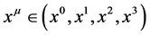
where, , (appearing in) run within and, , and. The spinor function represents

all family members of all the families.

The first line of Equation (2) determines (in) the kinematics and dynamics of spinor fields, coupled to the vector gauge fields. The generators of the charge groups are expressible in terms of through the complex coefficients, as presented in Equations ((34), (35), (39))

(3)

fulfilling the commutation relations

(4)

and representing the colour, the weak and the hyper charge. The corresponding vector gauge fields are expressible with the spin connection fields, with either or, in agreement with the assumptions ii. and iii.. In Subsection 2 the relation between the gauge fields, as obtain from the vielbeins in the ussual Kaluza-Klein procedure and those obtained from the spin connections as it is done in the spin-charge-family theory, is discussed. For a particular choice of the group (from) when vielbeins have a particular symmetry the proof that both procedures lead to the same vector gauge field in is presented. The expressions of the vector gauge fields goes for all the charges in a similar way as in this particular case (Equation (10)).

All vector gauge fields, appearing in the first line of Equation (2), except and (,is defined in Equation (39), in Equation (35)), are massless before the electroweak break. carries the colour charge (originating in), carries the weak charge (and are the subgroups of) and (,is defined in Equation (39), the corresponding group originates in, is defined in Equation (41) if the scalar space index s is replaced by the space vector index m, and is the third component of the second field). The fields and get masses of the order of the condensate scale through the interaction with the condensate of the two right handed neutrinos with the quantum numbers of the upper four families (the assumption iv., Table 1).

The condensate, Table 1, gives masses of the order of the scale of its appearance also to all the scalar gauge fields, presented in the second and the third line of Equation (2).

The charges () of the gauge fields are before the electroweak break the conserved charges, since the corresponding vector gauge fields don’t interact with the condensate. After the electroweak break, when the scalar fields with the space index―those with the family quantum numbers and those with the quantum numbers ()―start to self interact (Equation (21)) gaining nonzero vacuum expectation values, the weak charge and the hyper charge are no longer conserved. The only conserved charges are then the colour and the electromagnetic charges.

In Equations ((41), (40)) the scalar fields with the space index (7, 8), Equation (17), are presented as superpositions of the spin connection fields of both kinds. These scalar fields determine after the electroweak break the mass matrices of the two decoupled groups of four families (Equation (23)) and of the heavy bosons (Equation (24)).

Quarks and leptons have the “spinor” quantum number (, originating in (Equation (35), presented in Table 3) equal to and, respectively⁴ (with the sum of both equal to).

Let us conclude this Subsection with the recognition that:

A. It is (only) one scalar condensate of two right handed neutrinos (Table 1), which gives masses to all the vector and the scalar gauge fields appearing in the spin-charge-family theory, except to those vector gauge fields which enter into the standard model as massless vector gauge fields (the gravity, the colour vector gauge fields, the weak vector gauge fields and the hyper gauge field, the last three gauge fields manifesting after the electroweak break as the heavy bosons and the massless colour and electromagnetic gauge fields).

B. There are (only) the nonzero vacuum expectation values of the scalar gauge fields with the space index (with the weak charge equal to and the hyper charge correspondingly equal to, both due

to the space index), and with the family (twice two triplets) and family member quantum numbers (three singlets) in adjoint representations, which cause the electroweak break breaking the weak and the hyper charge symmetry.

The rest of the scalar fields, the members of the weak doublets (Table 2) with the space index, and the colour triplets and antitriplets with the space index [1] which contribute to transitions of antiparticles into particles and to proton decay, keep masses of the condensate scale.

Correspondingly the (only) two assumptions, iv. and v., make at the low energy regime observable the measured vector and scalar gauge fields, offering in addition the explanation also for the dark matter and the matter-antimatter asymmetry.

2. Relation between Spin Connections and Vielbeins When No Sources Are Present

It is demonstrated in this section for the case of spaces with no fermion sources present and with the symmetry of the vielbeins with the space indices () equal to, for any f, that both procedures―the ordinary Kaluza-Klein one with vielbeins and the procedure with spin connections used in the spin-charge-family theory―lead to the same gauge vector fields in.

Let us assume the infinitesimal coordinate transformations of the kind [13]

(5)

where we have made a choice of the symmetry

(6)

, and concern internal degrees of freedom of boson and fermion fields. The commutation relations for the generators of the groups (in this case),

, lead for the generators and to the commutation relations presented in Equations ((3), (4)) with.

It follows for the vielbeins representing the background field

(7)

The background field in is chosen to be flat, while the vielbeins represent the appearance of the vector gauge fields and in. Both fields are functions of the coordinates in only. We make a choice [13]

(8)

where and are the gauge fields of the charges and, respectively, depending on the coordinates only .

From it follows

(9)

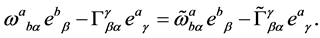
Statement: These two vector gauge fields are just the superposition of as used in the spin-charge-family theory:

(10)

To prove this statement let us express the operators, appearing in Equation (5), as follows

(11)

(One notices that.)

Then we use the relation between the fields and the vielbeins (Equation (62)), which in the case of no fermion sources present simplifies to

(12)

Let us now put the vielbeins from Equation (8) into the expressions for the gauge fields, let say (Equation (10)), expressing and with the right hand side of Equation (12). Taking into account the symmetry of the space of the coordinates, manifesting in, for any f (from where it follows that), one obtains after a little longer calculations that

(13)

Repeating equivalent calculations for the rest of components of and one obtains that:, and, what completes the proof.

3. Scalar Fields Contributing to Electroweak Break Belong to Weak Charge Doublets

It is proven in this section that all the scalar gauge fields with the space index carry―with respect to the space index s―the weak and the hyper charge as does the Higgs’s scalar of the standard model. These scalar fields, belonging either to (one of two times two) triplets with respect to the family quantum numbers or to (one of the three) singlets with respect to the family members quantum numbers, offer the explanation for the origin of the Higgs’s scalar and the Yukawa coupling of the standard model.

It turnes out [1] that all scalars (the gauge fields with the space index) of the action (Equation (1)) carry charges in the fundamental representations: They are either doublets (Table 2) or triplets [1] with respect to the space index. The scalars with the space indices and are the doublets (Table 2).

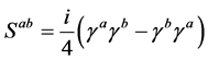
To see this one must take into account that the infinitesimal generators,

(14)

determine spins of spinors, while,

(15)

determine family charges of spinors (Equation (15)), while (Equation (47)), which apply on the spin connections () and (), on either the space index e or any of the indices operates as follows

(16)

in accordance with the Equations ((71)-(73)). Expressions for the infinitesimal operators of the subgroups of the starting groups (presented in Equations ((33)-(39))) are equivalent (have for the chosen the same coefficients in Equation (3)) for all three kinds of degrees of freedom (Appendix A2.1, Appendix A1).

All scalars carry correspondingly, besides the quantum numbers determined by the space index, also the quantum numbers, the states of which belong to the adjoint representations. At the electroweak break all the scalar fields with the space index (7, 8), those which belong to one of twice two triplets carrying the family quantum numbers (, Equations ((36)-(38))) and those which belong to one of the three singlets carrying the allowed family members quantum numbers (), Equation (39), Section 1.1, the assumption v. and the corresponding comments), start to self interact, Equation (21). Gaining nonzero vacuum expectation values they break the weak, the hyper charge and the family charges.

Statement: Scalar fields with the space index (7, 8) carry with respect to this space index the weak and the hyper charge (,), respectively.

To prove this statement let me introduce a common notation for all the scalar fields, independently of whether they originate in scalar fields―in this case―or in scalar fields―in this case all the family quantum numbers of all eight families contribute.

(17)

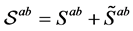
Here represent all the operators, which apply on the spinor states. These scalars, the gauge scalar fields of the generators and (Equations (35)-(37)), are expressible in terms of the spin connection fields (Equations ((40), (41))).

Let us make a choice of the superposition of the scalar fields so that they are eigenstates of

(Equation (34), if is replaced by) for all quantum numbers. Such a superpo-

sition appears by itself if one rewrites the second line of Equation (2) as follows (the momentum is left out⁵)

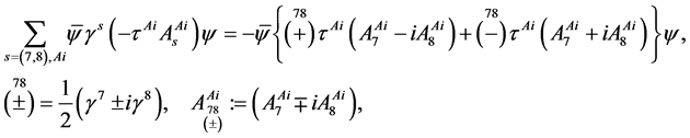(18)

with the summation over performed, since represent the scalar fields (, , , , , , and).

The application of the operators (Equations ((16), (39))) and (Equation (34), if is replaced by) on the fields gives

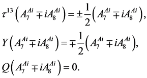(19)

Since, , and give zero, if applied on (,and) with respect to the indices (), and since and commute with the family quantum numbers, one sees that the scalar fields

(=, , , , , , , ,), rewritten as, are eigenstates of and, having the quantum numbers of the standard model Higgs’ scalar.

These superpositions of are presented in Table 2. Table 2 represents two doublets with respect to the weak charge, with the eigenvalue of (the second charge), Equation (34), if is replaced

by), equal to, respectively.

The operators (Equation (34), if is replaced by),

(20)

transform one member of a doublet from Table 2 into another member of the same doublet, keeping unchanged.

This completes the proof of the above statement.

After the appearance of the condensate (Table 1), which breaks the symmetry (bringing masses to all the scalar fields), the weak and the hyper charge remain the conserved charges⁶.

At the electroweak break the scalar fields with the space index (7, 8) start to interact among themselves so that the Lagrange density for these gauge fields changes from to

(21)

where and manifests as the mass of the scalar.

The operator (Equation (20)) transforms into, while

Let me pay attention to the reader, that the term in Equation (18) transforms the right

handed quark from the first line of Table 3 into the left handed quark from the seventh line of the same table⁷, which can, due to the properties of the scalar fields (Equation (19)), be interpreted also in the standard model way, namely, that “dress” giving it the weak and the hyper charge of the left handed

quark, while changes handedness. Equivalently happens to from the 25^th line, which transforms under

the action of into from the 31^th line.

The operator transforms from the third line of the Table 3 into from the fifth line of this table, or from the 27^th line into from the 29^th line, where belong to the scalar fields from Equation (17).

The term of the action (Equations ((1), (18))) takes care of the Yukawa couplings as well. All the scalar fields, presented in Equation (17), carry the weak and the hyper charge (Equations ((34),

(35))) of the Higgs of the standard model. If represents the first three operators in Equation (17) then it only multiplies the right handed family member with its eigenvalue. If represents the last four operators of

the same equation, then the operators (() for and, respectively) transform the right handed family member of one family into the left handed partner of another family within the same group of four families, since these four operators manifest the symmetry twice ().

The nonzero vacuum expectation values of the scalar fields of Equation (17) break the mass protection mechanism of quarks and leptons and determine correspondingly the mass matrices (Equation (23)) of the two groups of quarks and leptons. One group of four families carries the family quantum numbers (,), the other group of four families carries the family quantum numbers (,).

In loop corrections all the scalar and vector gauge fields which couple to fermions contribute. Correspondingly all the off diagonal matrix elements of the mass matrix (Equation (23)) depend on the family members quantum numbers.

It is not difficult to show that the scalar fields are triplets as the gauge fields of the family quantum numbers (, , ,; Equations ((16), (36), (37))) or singlets as the gauge fields of, and.

Let us do this for and for, taking into account Equation (33) (where we replace by) and Equation (16), and recognizing that.

One finds

(22)

with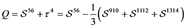, and with defined in Equation (35), if replacing by from Equation (16).

Similarly one finds properties with respect to the quantum numbers for all the scalar fields.

The mass matrix of any family member, belonging to any of the two groups of the four families, manifests - due to the (either () or ()) structure of the scalar fields, which are the gauge fields of and―the symmetry presented in Equation (23).

(23)

Let us summarize this section: It is proven that all the scalar fields with the scalar index, which at the electroweak break start to mutual interact and gain nonzero vacuum expectation values (Equation (21)), keeping the electromagnetic charge conserved, carry the weak and the hyper charge quantum numbers as required

by the standard model for the Higgs’s scalar (Equation (19)):. These are the only

scalar fields in this theory with the quantum numbers of the Higgs’s field. These scalar fields carry additional quantum numbers: The triplet family quantum numbers and the singlet family members quantum numbers and form two groups of four families. They all contribute to masses of the heavy bosons ([4] , Equation (53)) (,), reproducing on the tree level the expression for the mass term in the standard model

(24)

where are the contribution to the vacuum expectation value of all the scalar fields from Equation (19).

All the other scalar fields: and have masses of the order of the condensate scale and contribute to matter-antimatter asymmetry [1] .

3.1. Triplets with Respect to Space Index s = (9, ∙∙∙, 14)

The gauge fields with the space index form the triplets and antitriplets with respect to the space index. They are discussed in Ref. [1] . The colour triplet scalars contribute to transition from antileptons into quarks and antiquarks into quarks and back, unless the scalar condensate of the two right handed neutrinos, presented in Table 1, breaks matter-antimatter symmetry [1] , offering the explanation for the matter-antimatter asymmetry in our universe. This condensate leaves massless besides gravity only the colour, weak and the hyper charge vector gauge fields. Also all the scalar fields get masses through the interaction with the condensate.

There are no additional scalar indices and therefore no additional corresponding scalars with respect to the scalar indices in this theory.

Scalars, which do not get nonzero vacuum expectation values, keep masses on the condensate scale.

4. Vectors, Tensors and Spinors in Spin-Charge-Family Theory

This section discusses properties of vectors, tensors and spinors, appearing in the action in Equation (1), for -dimensional space-time, for any d in purpose to clarify the degrees of freedom of these fields, connected with the two kinds of the Clifford algebra objects: and (Equations ((47), (49))).

The presentation is based on Refs. [7] [6] [19] -[21] , where the two kinds of the Clifford objects’s and’s were introduced. In Ref. [7] these two kinds of the Clifford algebra objects were introduced in Grassmann space of anticommuting coordinates. A part of this reference is briefly repeated in Appendix A2, where’s and’s are introduced as two superposition of a coordinate and its momentum (Equation (47)).

(25)

where represents.

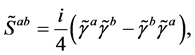
The Clifford algebra objects have properties (Equation (49))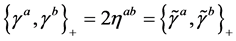, , 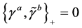while the generators of the infinitesimal Loorentz transformations fulfil the relations of Equation (50): , equivalent commutation relations are valid also for and, while.

Either the coordinates or the corresponding momenta transform as vectors with respect to the Lorentz transformations in the tangent space (Equation (43)) and so do and and correspondingly also, (Equation (53)).

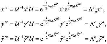(26)

where are parameters of transformations and is the operator of a finite Lorentz transformations. The Grassmann coordinate transforms correspondingly as:

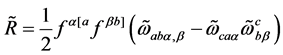We see that, , and transform as vectors, and are scalars and and, which appear in Equation (1) (are the vielbeins), are also scalars.

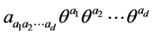
The linear vector space over the coordinate Grassmann space has the dimension (Subsection 7.2). Any vector in Grassmann space can be presented as written in Equation (45). Any complex number and

, where is an antisymmetric tensor, are scalars with respect to the Lorentz transformations.

Grassmann coordinates in Equation (45) can be replaced by one of the Clifford algebra objects, let say by, and correspondingly the linear vector space can as well be described by the polynomials as follows

(27)

provided that operation of and on such a vector space is understood as the left and the right multiplication (Equation (64))

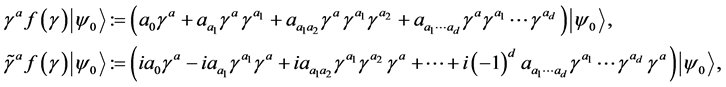(28)

where is a vacuum state.

With this definition the relations from Equations ((47), (50)-(53)) remain valid. If determine family quantum numbers, then transform spinor states within one family (Table 3), keeping family quantum numbers unchanged, while transform a family member of one family into the same family member of another family (Table 4).

It is still true that the infinitesimal generators of the Lorentz transformations for vectors are (Equation (47)), provided that we respect the rule of Equation (28). One correspondingly easily finds that any constant and the operator of handedness (Equation (68)) are the two scalars with respect to, in any d. In, for example, one finds [7] besides the two scalars (a constant and a product of all) also two three vectors and two four vectors.

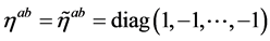
The two tangent spaces have the same metric tensors: and correspondingly for the Lorentz vectors, , or any two vectors and one finds that and.

Let us transform any two vectors and into the corresponding coordinate (curved) space with the vielbeins

(29)

Here and.

In Appendix A3 relations among the vielbeins and the two kinds of the spin connection fields, and, which are the gauge fields of and, respectively, are studied under the assumption that space-time has a structure of a differentiable manifold [13] . The relation among the two kinds of

the spin connection fields, and (Equations ((54), (55))), and the corresponding two kinds of the affine connections, and (Equations ((56), (57))), is presented. The requirement that the covariant de-

rivative of the vielbeins is equal to zero (Equation (60)) relates the two affine connections, and, with the two spin connections, and,

(30)

Varying the action in Equation (1) with respect to leads to the equations of motion

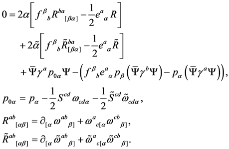(31)

Variation of the action with respect to and, respectively, in the presence of the spinor fields leads [22] to the two equations

(32)

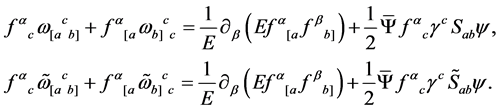
One notices from Equations ((31), (32)) that if there are no spinor sources, then both spin connections―and―are expressible with the vielbeins in the same way and correspondingly equal to each other. Then also and are equal (Equation (61). The only propagating fields are in this case the vielbeins.

The expressions for the two spin connection fields [22] , and, as functions of the vielbeins and the spinor sources are presented in Equation (62). If there are spinors present, then in general the two kinds of the spin connection fields are different.

The condensate (Table 1) of two right handed neutrinos, with the quantum numbers of the eighth family, contributes differently to than to. It influences also. In a flat space, that is with vielbeins equal to, the condensate (independent of all coordinates) contributes to different spin connection fields (like, , and several others) different constants.

5. Conclusions

It is demonstrated in this paper (Section 3) that all the scalar gauge fields of the starting action (the second line in Equation (2)) of the spin-charge-family theory [1] -[11] with the space index are, before the electro-

weak break, members of the two weak doublets (Table 2) with the hyper charge, respectively.

These scalars (Equation (17)) interact besides through the weak and the hyper charge (determined by the space index) either through the family quantum numbers―they belong to twice two triplets (either to or to) carrying the quantum numbers of either (,) or (,), respectively―or through the family members quantum numbers―()―as singlets. Triplets are the gauge scalar fields of the Clifford algebra objects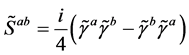, while singlets are the scalar gauge fields of the Clifford algebra objects (4) [7] .

Correspondingly they either transform members of one group of four families of fermions among themselves, keeping the family member quantum number unchanged, or interact with each family member according to their eigenvalues of the family members charges (), keeping the family quantum numbers unchanged.

When these scalars start to interact among themselves (Equation (21)), they gain nonzero vacuum expectation values, break the weak and the hyper charge, while preserving the electromagnetic charge, and cause the electroweak break. They determine mass matrices (Equation (23)) of two groups of four families as well as masses of the heavy bosons (Equation (24)).

These scalar fields with the space index and correspondingly with the weak charge and the hyper charge and all the family charges in the adjoint representations offer an explanation for the appearance of the Higgs’s scalar fields and the Yukawa couplings.

The paper discusses the relation between the Kaluza-Klein way through vielbeins and the spin-charge-family way through spin connections when explaining the appearance of the vector gauge fields in. It is proven in Section 2 that, when there are no spinor sources present and the space exhibits in a large enough symmetry so that vielbeins in have the property for any choice of f; both ways lead to the same vector gauge fields.

The paper discusses also the Lorentz properties of the scalar and vector gauge fields of this theory―the vielbeins and the two kinds of the spin connection fields―showing up the difference among all three kinds of the gauge fields in the presence of the spinor sources, while in the absence of the spinor sources only one of these three kinds of gauge fields is the propagating field (Section 4, and Appendix A2, Appendix A3).

All the scalar and vector gauge fields, and all the family members and the families appearing in this theory have the interpretation in the observed fermion and boson fields.

The theory predicts two decoupled groups of four families [4] [5] [10] [11] : The fourth of the lower group of families will be measured at the LHC [12] and the lowest of the upper four families constitutes the dark matter [11] . It also predicts that there will be several scalar fields observed sooner or later at the LHC, and that there is a new nuclear force among the fifth (and also the rest three of the upper group of four families) family baryons. The condensate contributes to the dark energy, as it does also the nonzero vacuum expectation values of the scalar fields with the space index (7, 8).

Let me conclude with pointing out that the spin-charge-family theory is offering a possible next step beyond the standard model by offering the explanation for all the assumptions of the standard model and also so far to several phenomena of the cosmology, which are not yet understood: the dark matter [11] , the matter/antimatter asymmetry [1] . The spin-charge-family theory essentially differs from the unifying theories of Pati and Salam [18] , Georgi and Glashow [23] and other and theories [24] , and also from the Kaluza-Klein theories [25] [26] , although all these unifying theories have many things in common―among themselves and with the spin-charge-family theory.

There are a lot of open questions in the elementary particle physics and cosmology which wait to be answered in addition to those presented in this paper. To see whether the spin-charge-family can offer answers also to (some) of those questions remains so far the open question.

Acknowledgements

The author acknowledges funding of the Slovenian Research Agency, which terminated in December 2014.

Cite this paper

Norma Susana MankočBorštnik, (2015) The Explanation for the Origin of the Higgs Scalar and for the Yukawa Couplings by the Spin-Charge-Family Theory. Journal of Modern Physics,06,2244-2274. doi: 10.4236/jmp.2015.615230

References

Appendix A1. Standard Model Subgroups of Group, Subgroups of Group and Corresponding Gauge Vector and Scalar Fields

This section follows the similar section in Refs. [1] [4] . To calculate quantum numbers of one Weyl representation presented in Table 3 in terms of the generators of the standard model groups , Equation (3), one must look for the coefficients. The generators are the generators of the charge groups: (originating in), (originating in), (originating in), (originating in) and (originating in). Equivalently the generators of the family subgroups of the group are defined and expressed.

I present here also the gauge fields to the corresponding either the spins and charges or to the family quantum numbers in terms of either or, respectively.

For a chosen group the same coefficients determine generators of all three kinds of quantum numbers: Of those applying either on the family member or on the family quantum number of spinors, or on quantum numbers of bosons (of the vector and the scalar gauge fields). The difference among these three kinds of operators comes from the generators in d-dimensional space: (for spins, Equation (14)), (for family quantum numbers, Equation (15)) and (for quantum numbers of gauge fields, Equation (16)).

While for spins of spinors is equal to, and for families of spinors is equal to is, which applies on the spin connections and , on either the space index e or the indices, equal to , or equivalently, in the matrix notation, . This means that the space index (e) of transforms according to the requirement of Equation (16), and so do and. I used the notation to point out that and are generators of two independent groups.

One finds [2] -[9] [27] for the infinitesimal generators of the spin and the charge groups, which are the subgroups of, the expressions:

(33)

where the generators determine representations of the two invariant subgroups of, the generators and,

(34)

determine representations of the invariant subgroups of the group, which is further the subgroup of (and are subgroups of), and the generators,.

(35)

determine representations of, originating in.

One correspondingly finds the generators of the subgroups of,

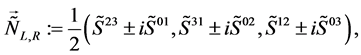(36)

which determine representations of the two invariant subgroups of, while

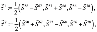(37)

determine representations of of. Both, and, are the subgroups of. One finds for the infinitesimal generator of originating in the expression

(38)

The corresponding expressions for the generators of the above subgroups defining the representations of the corresponding gauge fields follow if replacing or by from (Equation (16)).

One further defines the operators for the charges and of the standard model, together with and, and the corresponding operators of the family charges, , ,

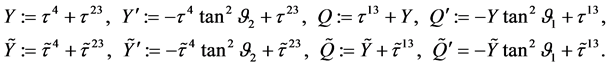(39)

The corresponding operators which apply on the corresponding gauge fields follow from the above relations, if either or are replaced by from Equation (16).

The scalar fields, responsible [2] -[4] ―after gaining nonzero vacuum expectation values and triggering the electroweak break―for masses of the family members and of the heavy bosons, are presented in the second line

of Equation (2). These scalar fields are included in the covariant derivatives as, , , , 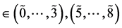where notation is again used to point out that belong in this case to the “tilde” space.

One finds the scalar fields carrying the quantum numbers of the subgroups of the family groups, expressed in terms of (they contribute to mass matrices of quarks and leptons and masses of the heavy bosons), if taking into account Equations ((36), (37), (39)),

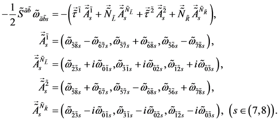(40)

The expressions for the scalars, expressed in terms of (contributing as well to the mass matrices of quarks and leptons and to masses of the heavy bosons) follow, if using Equations ((34), (35), (39))

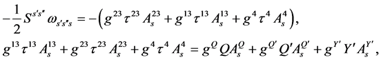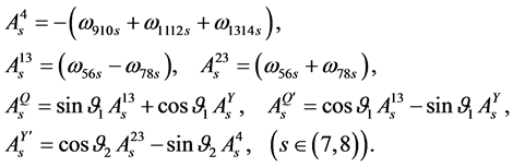(41)

(41)

Scalar fields from Equation (40) couple to the family quantum numbers, while those from Equation (41) couple to the family members quantum numbers. In Equation (41) the coupling constants are explicitly written in order to see the analogy with the gauge fields of the standard model.

Expressions for the vector gauge fields in terms of the spin connection fields and the vielbeins, which correspond to the colour charge (), the charge (), the weak charge () and the charge originating in (), can be found by taking into account Equations ((34), (35)). Equivalently

one finds the vector gauge fields in the “tilde” sector, or one just uses the expressions from Equations ((41), (40)), if replacing the scalar index s with the vector index m.

Appendix A2. Symmetries of Vectors, Tensors and Spinors

In this section the Lorentz transformations of’s,’s and correspondingly of vector, tensor and spinor fields in -dimensional space-time are discussed. The presentation is based on the papers [6] [7] , where the two kinds of the Clifford objects’s,’s were introduced (in those papers the notation and, respectively, was used, the present notation―and―was introduced in Refs. [19] -[21] ). Ref [7] starts with the Grassmann space of anticommuting coordinates. I do the same in Subsection 7.1. The two kinds of the Clifford algebra objects (Equations ((63), (64))) in the Grassmann space are introduced in Subsection 7.2 as the two superposition of a Grassmann coordinate and its derivative and their properties are discussed, as well as the Lorentz transformations of and and of any vector or tensor.

One could start instead with the two kinds of the Clifford algebra objects, without using the Grassmannn space, as it is presented in Appendix A4 and explained in Section 4, Equation (27).

Appendix A2.1. Coordinate Space with Grassmann Character and Lorentz Transformations

I shall repeat here some properties of the anticommuting Grassmann coordinates, since the appearance of the two kinds of the Clifford algebra objects can in the Grassmann space easily be demonstrated.

A point in d-dimensional Grassmann space of real anticommuting coordinates, ,

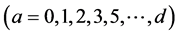(42)

is determined by a vector. The metric tensor () lowers the indices of a vector:. A Lorentz transformation on a vector component and on a vector component, which is a real (ordinary) commuting coordinate,

(43)

leaves forms

(44)

invariant. While is a symmetric tensor made of complex numbers, is an antisymmetric tensor made of complex numbers. The requirements that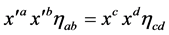, and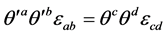, is the antisymmetric tensor, lead to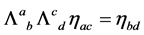. An infinitesimal Lorentz transformation for the case with can be written as, where.

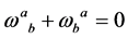Appendix A2.2. Linear Vector Space and Linear Operators over Coordinate Grassmann Space

A linear vector space over the coordinate Grassmann space has the dimension, due to the fact that for any.

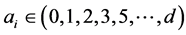Any vector in this space can be presented as a linear superposition of monomials

(45)

The left derivative on vectors of the space of monomials is defined as follows

(46)

The linear operators, and, , and are defined as

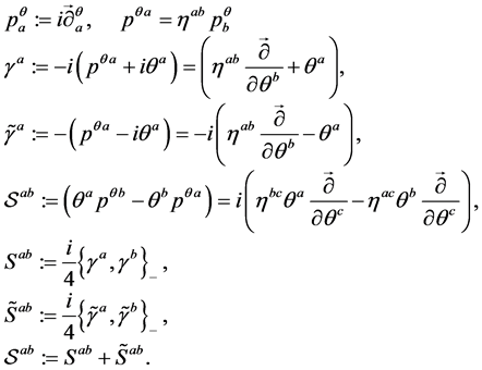(47)

means.

The factors in front of the superposition of and in the second and the third line of Equation (47) are chosen so that both Clifford algebra objects, and, fulfil the same Clifford algebra relation (the third and the fourth line in Equation (49)). One finds

(48)

and equivalently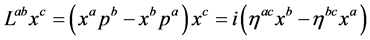. It follows

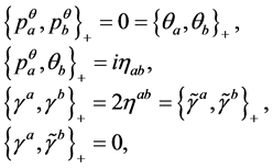(49)

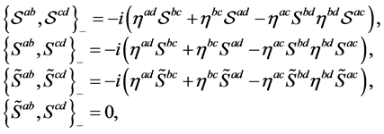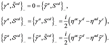(50)

(50)

An infinitesimal Lorentz transformation of the proper ortochronous Lorentz group is then

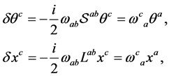(51)

where are parameters of a transformation.

Let us write the operator of finite Lorentz transformations as follows

(52)

We see that the coordinates and and the operators and transform as vectors Equation (26)

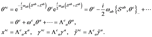(53)

Correspondingly one finds that compositions like and, here are , transform as scalars (remaining invariants), while and transform as vectors: ,.

Also objects like and 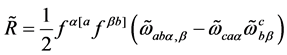from Equation (1) transform with respect to the Lorentz transformations as scalars.

Appendix A3. Spin Connection Fields of Two Kinds and Vielbeins in Presence of Spinor Sources [22]

Relations among the vielbeins and both kinds of the spin connection fields, and, which are the gauge fields of and, respectively, are studied under the assumption that space-time has a structure of a differentiable manifold [13] .

The two kinds of vectors, and, belonging to two different tangent spaces, transform with respect to the Lorentz transformations according to Equation (53).

We express, after the parallel transport⁸ of each of these two kinds of vectors (belonging to two tangent spaces) from to, in terms of the two kinds of the spin connections, and, respectively, as follows

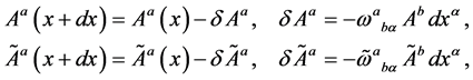(54)

where and are the two spin connection fields, related to tangent spaces. Requiring for the metric tensors, and, that they are the same at each point of each of the two tangent spaces, the relations 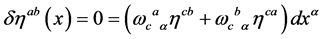and follow, which demonstrate the antisymmetry property of both spin connections: 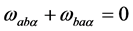and. Taking into account Equation (47) it must be that.

The difference between the two vectors and, is obtained by the differentiation, follows from the parallel transport, defines the covariant derivative of the vector in the tangent space:

, where. Equivalently one obtains the covariant derivative of the vector:.

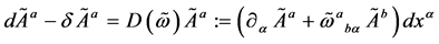(55)

We define the parallel transport also for the two kinds of vectors and (and) by introducing two kinds of the affine connections and, respectively,

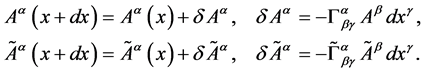(56)

The difference between the two vectors and, and equivalently between the two vectors and, defines the covariant derivatives of the vector and of the vector

(57)

The affine connection (as well as the “tilde affine connection”) can be expressed by the torsion (and the “tilde torsion”) and the Christoffel connection (,)

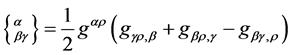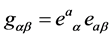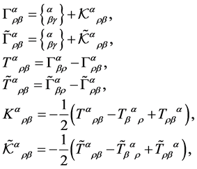(58)

and are the two contorsion tensors [13] . One finds

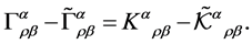(59)

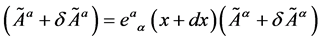When requiring that and, and correspondingly relating two kinds of different coordinate systems for either or, we find the related covariant derivatives

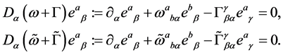(60)

Equation (60) relates the two affine connections, and, with the two spin connections and

(61)

Let us now vary the action Equation (1) with respect to and, respectively, in the presence of the spinor fields. One ends up [22] with the two expressions presented in Equation (32). Let me point out that if there are no spinor sources, then both spin connections―and―are expressible with the vielbeins

in the same way. Only one of these three fields are in this case the propagating field. Correspondingly also and are expressible with the vielbeins.

Multiplying both equations of Equation (32) by and summing over both indices, the expressions for and follow.

The expression for the spin connection and can [22] then easily be found

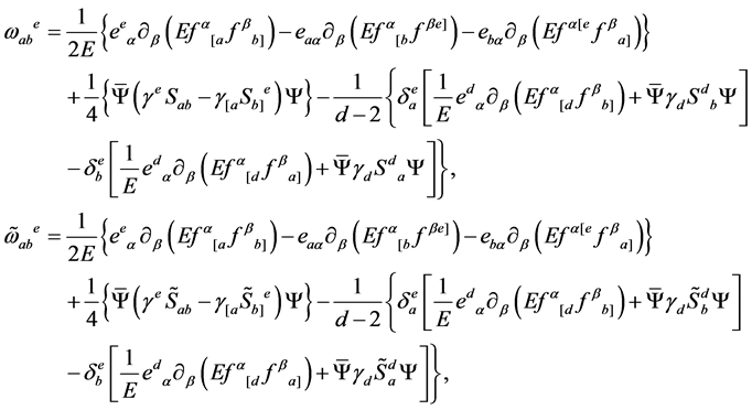(62)

Again one notices that if there are no spinor sources, carrying the spinor quantum numbers and for all, then and are completely determined by the vielbeins. In general both kinds of spinor sources affect the spin connections and vielbeins in their own way, making all three fields, vielbeins and both kinds of the spin connection fields, propagating fields.

Variation of the action Equation (1) with respect to leads to the equations of motion Equation (31).

Appendix A4. Short Presentation of Spinor Technique [4] [7] [20] [21]

This appendix is a short review (taken from [4] ) of the technique [7] [19] -[21] , initiated and developed in Ref. [7] , while proposing the spin-charge-family theory [1] - [12] [27] . All the internal degrees of freedom of spinors, with family quantum numbers included, are describable in the space of d-anticommuting (Grassmann) coordinates [7] , if the dimension of ordinary space is also d (Appendix A4). There are two kinds of operators in the Grassmann space fulfilling the Clifford algebra and anticommuting with one another 4, Equation (47). The technique was further developed in the present shape together with H.B. Nielsen [19] -[21] .

In this last stage we rewrite a spinor basis, written in Ref. [7] as products of polynomials of Grassmann coordinates of odd and even Grassmann character, chosen to be eigenstates of the Cartan subalgebra defined by the two kinds of the Clifford algebra objects, as products of nilpotents and projections, formed as odd and even objects of’s, respectively, and chosen to be eigenstates of a Cartan subalgebra of the Lorentz groups defined by’s and’s.

The technique can be used to construct a spinor basis for any dimension d and any signature in an easy and transparent way. Equipped with the graphic presentation of basic states, the technique offers an elegant way to see all the quantum numbers of states with respect to the two Lorentz groups, as well as transformation properties of the states under any Clifford algebra object.

Appendix A2 briefly represents the starting point [7] of this technique in order to better understand the Lorentz transformation properties of both Clifford algebra objects,’s and’s, as well as of spinor, vector, tensor and scalar fields, appearing in the spin-charge-family theory, that is of the vielbeins and spin connections of both kinds, and, and of spinor fields, family members and families.

The objects and have properties (49),

(63)

If B is a Clifford algebra object, let say a polynomial of (Equation (27)), , one finds

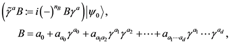(64)

where is a vacuum state, defined in Equation (78) and is equal to 1 for the term in the polynomial which has an even number of’s, and to −1 for the term with an odd number of’s, for any d, even or odd, and I is the unit element in the Clifford algebra.

It follows from Equation (64) that the two kinds of the Clifford algebra objects are connected with the left and the right multiplication of any Clifford algebra objects B (Equation (28)).

The Clifford algebra objects and close the algebra of the Lorentz group (Equation (50))

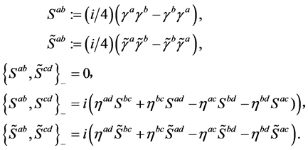(65)

We assume the “Hermiticity” property for’s

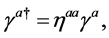(66)

in order that are compatible with (63) and formally unitary, i.e..

One finds from Equation (66) that.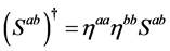

Recognizing from Equation (65) that the two Clifford algebra objects with all indices different commute, and equivalently for, we select the Cartan subalgebra of the algebra of the two groups, which form equivalent representations with respect to one another

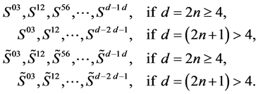(67)

The choice for the Cartan subalgebra in is straightforward. It is useful to define one of the Casimirs of the Lorentz group―the handedness in any d

(68)

One proceeds equivalently for, subtituting’s by’s. We understand the product of’s in the ascending order with respect to the index a:. It follows from Equation (66) for any choice of the signature that We also find that for d even the handedness anticommutes with the Clifford

algebra objects , while for d odd it commutes with .

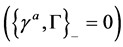To make the technique simple we introduce the graphic presentation as follows

(69)

where. It follows then

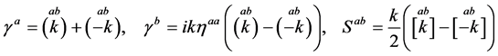(70)

One can easily check by taking into account the Clifford algebra relation (Equation (63)) and the definition of and (Equation (65)) that the nilpotent and the projector are “eigenstates” of and

(71)

which means that we get the same objects back multiplied by the constant in the case of, while multiply by k and by rather than. This also means that when and act from the left hand side on a vacuum state the obtained states are the eigenvectors of. We further recognize that transform into, never to, while transform into, never to

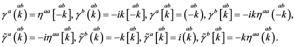(72)

From Equation (72) it follows

(73)

From Equation (73) we conclude that generate the equivalent representations with respect to and opposite.

Let us deduce some useful relations

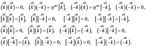(74)

We recognize in Equation (74) the demonstration of the nilpotent and the projector character of the Clifford algebra objects and, respectively. Defining

(75)

one recognizes that

(76)

Recognizing that

(77)

we define a vacuum state so that one finds

(78)

Taking into account the above equations it is easy to find a Weyl spinor irreducible representation for d-dimensional space, with d even or odd.

For d even we simply make a starting state as a product of d/2, let us say, only nilpotents, one for each

of the Cartan subalgebra elements (Equation (67)), applying it on an (unimportant) vacuum state. For d odd the basic states are products of nilpotents and a factor. Then the generators, which do not belong to the Cartan subalgebra, being applied on the starting state from the left, generate all the members of one Weyl spinor.

(79)

All the states have the same handedness, since. States, belonging to one multiplet with re-

spect to the group, that is to one irreducible representation of spinors (one Weyl spinor), can have any phase. We made a choice of the simplest one, taking all phases equal to one.

The above graphic representation demonstrates that for d even all the states of one irreducible Weyl representation of a definite handedness follow from a starting state, which is, for example, a product of nilpotents, by transforming all possible pairs of into. There are, which do this. The procedure gives states. A Clifford algebra object being applied from the left hand side, transforms a Weyl spinor of one handedness into a Weyl spinor of the opposite handedness. Both Weyl spinors form a Dirac spinor.

We shall speak about left handedness when and about right handedness when for either d even or odd.

While which do not belong to the Cartan subalgebra (Equation (67)) generate all the states of one representation, which do not belong to the Cartan subalgebra (Equation (67)) generate the states of equivalent representations.

Making a choice of the Cartan subalgebra set (Equation (67)) of the algebra and , , , , , , , , , , , , , a left handed () eigenstate of all the members of the Cartan subalgebra, representing a weak chargeless -quark with spin up, hyper

charge (2/3) and colour, for example, can be written as

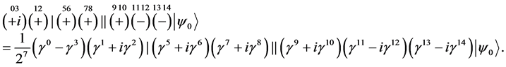(80)

This state is an eigenstate of all and which are members of the Cartan subalgebra (Equation (67)).

The operators, which do not belong to the Cartan subalgebra (Equation (67)), generate families from the starting quark, transforming the quark from Equation (80) to the of another family, keeping all of the properties with respect to unchanged. In particular, applied on a right handed -quark from Equation (80) generates a state which is again a right handed -quark, weak chargeless, with spin up, hyper

charge (2/3) and the colour charge

(81)

Below some useful relations [5] are presented

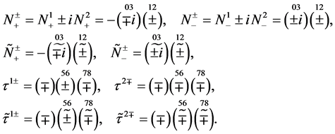(82)

I present at the end one Weyl representation of and the family quantum numbers of the two groups of four families.

One Weyl representation of contains left handed weak charged and the second chargeless coloured quarks and colourless leptons and right handed weak chargeless and the second charged quarks and leptons (electrons and neutrinos). It carries also the family quantum numbers, not mentioned in this table. The table is taken from Ref. [16] .

The eight families of the first member of the eight-plet of quarks from Table 3, for example, that is of the right handed quark, are presented in the left column of Table 4 [4] . In the right column of the same table the equivalent eight-plet of the right handed neutrinos are presented. All the other members of any of the eight families of quarks or leptons follow from any member of a particular family by the application of the operators and on this particular member.

The eight-plets separate into two group of four families: One group contains doublets with respect to and, these families are singlets with respect to and. Another group of families contains doublets with respect to and, these families are singlets with respect to and.

The scalar fields which are the gauge scalars of and couple only to the four families which are

doublets with respect to these two groups. The scalar fields which are the gauge scalars of and couple only to the four families which are doublets with respect to these last two groups.

NOTES

¹In the spin-charge-family theory the weak and the hyper charge of the scalar fields originate in the invariant subgroups of (), having the analogue in the spin representation of the vector gauge fields in.

² are inverted vielbeins to with the properties,. Latin indices denote a tangent space (a flat index), while Greek indices denote an Einstein index (a curved index). Letters from the beginning of both the alphabets indicate a general index (and ), from the middle of both the alphabets the observed dimensions (and), indices from the bottom of the alphabets indicate the compactified dimensions (and). We assume the signature.

³A toy model [14] [15] was studied in with the same action as in Equation (1). The break from to an almost was studied. For a particular choice of vielbeins and for a class of spin connection fields the manifold breaks into times an almost, while families remain massless and mass protected. Equivalent assumption, although not yet proved how does it really work, is made in the case. This study is in progress.

⁴In the Pati-Salam model [18] this “spinor” quantum number is named quantum number and is twice the “spinor” quantum number, for quarks equal to and for leptons to.

⁵It is expected that solutions with nonzero momentum lead to higher masses of the fermion fields in d = (3 + 1) [14] [15] . We correspondingly pay no attention to the momentum, when having in mind the lowest energy solutions, manifesting at low energies.

⁶It is which determines the hyper charge (, Equation (39)) of these scalar fields, since applied on the scalar index of these scalar fields gives zero, according to Equations ((34), (35)) in which is replaced by from Equation (16).

⁷This transformation of the right handed family members into the corresponding left handed partners can easily be calculated by using Equation ((74), (72), (82)).

⁸In Ref. [13] the parallel transport is discussed at pages from 52-66.

References

- 1. Mankoc Borstnik, N.S. (2015) Physical Review D, 91, Article ID: 065004. [arxiv:1409.7791]
http://dx.doi.org/10.1103/PhysRevD.91.065004 - 2. Mankoc Borstnik, N.S. (2013) Spin-Charge-Family Theory Is Explaining Appearance of Families of Quarks and Leptons, of Higgs and Yukawa Couplings. Mankoc Borstnik, N.S., Nielsen, H.B. and Lukman, D., Eds., Proceedings to the 16th Workshop “What Comes beyond the Standard Models”, Bled, 14-21 July 2013, DMFA Zaloznistvo, Ljubljana, 113. [arxiv:1312.1542, arxiv:1409.4981]
- 3. Mankoc Borstnik, N.S. (2012) Do We Have the Explanation for the Higgs and Yukawa Couplings of the Standard Model. Mankoc Borstnik, N.S., Nielsen, H.B. and Lukman, D., Eds., Proceedings to the 15th Workshop “What Comes beyond the Standard Models”, Bled, 9-19 of July 2012, DMFA Zaloznistvo, Ljubljana, 56-71.
[arxiv:1302.4305,arxiv:1011.5765] - 4. Mankoc Borstnik, N.S. (2013) Journal of Modern Physics, 4, 823-847. [arxiv:1312.1542]
http://dx.doi.org/10.4236/jmp.2013.46113 - 5. Borstnik Bracic, A. and Mankoc Borstnik, N.S. (2006) Physical Review D, 74, Article ID: 073013.
[hep-ph/0301029; hep-ph/9905357, p. 52-57; hep-ph/0512062, p. 17-31; hep-ph/o401043, p. 31-57] - 6. Mankoc Borstnik, N.S. (1992) Physics Letters B, 292, 25-29.
http://dx.doi.org/10.1016/0370-2693(92)90603-2 - 7. Mankoc Borstnik, N.S. (1993) Journal of Mathematical Physics, 34, 3731.
http://dx.doi.org/10.1063/1.530055 - 8. Mankoc Borstnik, N.S. (2001) International Journal of Theoretical Physics, 40, 315-338.
http://dx.doi.org/10.1023/A:1003708032726 - 9. Mankoc Borstnik, N.S. (1995) Modern Physics Letters A, 10, 587.
http://dx.doi.org/10.1142/S0217732395000624 - 10. Bregar, G., Breskvar, M., Lukman, D. and Mankoc Borstnik, N.S. (2008) New Journal of Physics, 10, Article ID: 093002.
http://dx.doi.org/10.1088/1367-2630/10/9/093002 - 11. Bregar, G. and Mankoc Borstnik, N.S. (2009) Physical Review D, 80, Article ID: 083534.
http://dx.doi.org/10.1103/PhysRevD.80.083534 - 12. Bregar, G. and Mankoc Borstnik, N.S. (2003) Can We Predict the Fourth Family Masses for Quarks and Leptons? Mankoc Borstnik, N.S., Nielsen, H.B. and Lukman, D., Eds., Proceedings to the 16th Workshop “What Comes beyond the Standard Models”, Bled, 14-21 July 2013, DMFA Zaloznistvo, Ljubljana, 31-51. [arxiv:1403.4441]
- 13. Blagojevic, M. (2002) Gravitation and Gauge Symmetries. IoP Publishing, Bristol.
http://dx.doi.org/10.1887/0750307676 - 14. Lukman, D., Mankoc Borstnik, N.S. and Nielsen, H.B. (2011) New Journal of Physics, 13, Article ID: 103027.
http://dx.doi.org/10.1088/1367-2630/13/10/103027 - 15. Lukman, D. and Mankoc Borstnik, N.S. (2012) Journal of Physics A: Mathematical and Theoretical, 45, Article ID: 465401. [arxiv:1205.1714; arxiv:1312.541; hepph/0412208, p. 64-84]
http://dx.doi.org/10.1088/1751-8113/45/46/465401 - 16. Mankoc Borstnik, N.S. and Nielsen, H.B.F. (2014) Journal of High Energy Physics, 165. [arXiv:1212.2362]
http://dx.doi.org/10.1007/JHEP04(2014)165 - 17. Troha, T., Lukman, D. and Mankoc Borstnik, N.S. (2014) International Journal of Modern Physics A, 29, Article ID: 1450124. [arXiv:1312.1541]
http://dx.doi.org/10.1142/S0217751X14501243 - 18. Pati, J. and Salam, A. (1974) Physical Review D, 10, 275.
http://dx.doi.org/10.1103/PhysRevD.10.275 - 19. Mankoc Borstnik, N.S. and Nielsen, H.B. (2000) Physical Review D, 62, Article ID: 044010. [hep-th/9911032]
http://dx.doi.org/10.1103/PhysRevD.62.044010 - 20. Mankoc Borstnik, N.S. and Nielsen, H.B. (2002) Journal of Mathematical Physics, 43, 5782. [hep-th/0111257]
http://dx.doi.org/10.1063/1.1505125 - 21. Mankoc Borstnik, N.S. and Nielsen, H.B. (2003) Journal of Mathematical Physics, 44, 4817. [hep-th/0303224]
http://dx.doi.org/10.1063/1.1610239 - 22. Mankoc Borstnik, N.S., Nielsen, H.B. and Lukman, D. (2004) An Example of Kaluza-Klein-Like Theories Leading after Compactification to Massless Spinors Coupled to a Gauge Field-Derivations and Proofs. Mankoc Borstnik, N., Nielsen, H.B., Froggatt, C. and Lukman, D., Eds., Proceedings to the 7th Workshop “What Comes Beyond the Standard Models”, Bled, 19-31 July 2004, DMFA Zaloznistvo, Ljubljana, 64-84. [hep-ph/0412208]
- 23. Georgi, H. and Glashow, S. (1974) Physical Review Letters, 32, 438.
http://dx.doi.org/10.1103/PhysRevLett.32.438 - 24. Zee, A., Ed. (1982) Unity of Forces in the Universe. World Scientic, Singapore. arXiv:1403.2099 [hep-ph]
- 25. Lee, H.C., Ed. (1983) The Authors of the Works Presented in an Introduction to Kaluza-Klein Theories. World Scientic, Singapore.
Appelquist, T., Chodos, A. and Freund, P.G.O., Eds. (1987) Modern Kaluza-Klein Theories. Addison Wesley, Reading. - 26. Witten, E. (1981) Nuclear Physics B, 186, 412-428.
http://dx.doi.org/10.1016/0550-3213(81)90021-3 - 27. Borstnik, A. and Mankoc Borstnik, N.S. (2003) Weyl Spinor of SO(1, 13), Families of Spinors of the Standard Model and Their Masses. Mankoc Borstnik, N., Nielsen, H.B., Froggatt, C. and Lukman, D., Eds., Proceedings to the Euroconference on Symmetries beyond the Standard Model, Portoroz, 12-17 July 2003, DMFA, Zaloznistvo, Ljubljana, 31-57. [hep-ph/0401043; hep-ph/0401055]
Appendix A1. Standard Model Subgroups of
Group, Subgroups of
Group and Corresponding Gauge Vector and Scalar Fields