Journal of Modern Physics
Vol.3 No.9(2012), Article ID:22676,17 pages DOI:10.4236/jmp.2012.39127
Relativity Theory and Paraquantum Logic—Part II: Fundamentals of an Unified Calculation
1Group of Applied Paraconsistent Logic-Santa Cecília University, Santos, Brazil
2Institute for Advanced Studies of the University of São Paulo Cidade Universitária, São Paulo, Brazil
Email: inacio@unisanta.br
Received July 8, 2012; revised August 18, 2012; accepted August 28, 2012
Keywords: Paraconsistent Logic; Paraquantum Logic; Classical Physic; Relativity Theory; Quantum Mechanics
ABSTRACT
The studies of the PQL are based on propagation of Paraquantum logical states ψ in a representative Lattice of four vertices. Based in interpretations that consider resulting information of measurements in physical systems are found paraquantum equations for computation of the physical quantities in real physical systems. In the first part of this work we presented a study of Relativity theory which involved the time and the space with their characteristics as degrees of evidence applied in Paraquantum Logical Model. Now, in this second Part we present a study of application of the PQL in resolution of phenomena of physical systems that involve concepts of the Relativity Theory and the correlation of these effects with the Newtonian Universe and Quantum Mechanics. Considering physical fundamental quantities varying periodically in amplitude, we introduce the paraquantum equations which consider frequency in the analysis. From of these mathematical relationships obtained in the PQL Lattice some main physical constants related to the studies of De Broglie appeared. With the equations of Energy obtained through the analyses is demonstrated that the Paraquantum Logic is capable to correlate values and to unify the several study areas of the Physical Science.
1. Introduction
The Paraconsistent Annotated Logics with annotation of two values (PAL2v) is a class of Paraconsistent Logics particularly represented through a Lattice of four vertices (see [1-4]). The main feature of Paraconsistent Logic is the ability to accept contradiction and with fundamental concepts of the PAL2v was created the Paraquantum Logic (PQL) [5,6]. Through the paraquantum equations we investigate the effects of balancing of Energies and the quantization and transience properties of the Paraquantum Logical Model in real Physical Systems [6,7]. With study done at [4] were defined the values in a Lattice τ, representative of Paraconsistent Logic, where:
Certainty Degree (DC) on the x-axis is obtained by:
 , (1)
, (1)
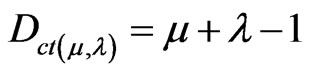
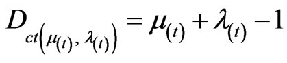
Contradiction Degree (Dct) on the y-axis is obtained by:
 , (2)
, (2)
where, according to the language of the PAL2v:
m → is the favorable Evidence Degree ( );
);
λ → is the unfavorable Evidence Degree ( ).
).
From (1) and (2) we can represent a Paraconsistent logical state eτ into Lattice τ of the PAL2v [4,5], such that:
 , (3)
, (3)
where:
eτ is the Paraconsistent logical state;
DC is the Certainty Degree obtained from the evidence Degrees μ and λ;
Dct is the Contradiction Degree obtained from the evidence Degrees μ and λ.
The values of the degrees of evidence are extracted from Observable Variables in the physical world. So, the variations in their physical characteristics are transmitted for analysis in the Lattice τ that represents the Paraconsistent world [4].
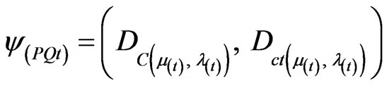
A Paraquantum logical state ψ is created on the lattice as the tuple formed by the Certainty degree (DC) and the Contradiction degree (Dct) [4].
 (4)
(4)
 (5)
(5)
Both values depend on the measurements perfomed on the Observable Variables in the physical environment which are represented by μ and λ [4,7,8]. For each measurement performed in the physical world of μ and λ, we obtain a unique duple  which represents a unique Paraquantum logical state ψ which is a point of the lattice of the PQL [4,7]. Then, a Paraquantum function y(Py) is defined as the Paraquantum logical state y:
On the vertical y-axis of contradictory degrees, the two extreme real Paraquantum logical states are:
1) Inconsistency T: 2) Undetermination ^:
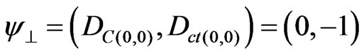 .
.
On the horizontal x-axis of certainty degrees, the two extreme real Paraquantum logical states are:
1) Veracity t: 2) Falsity F:
 .
.
A Vector of State  will have origin in one of the two vertexes that compose the horizontal axis of the certainty degrees and its extremity will be in the point formed for the pair indicated by the Paraquantum function
 .
.
If the Certainty Degree is negative (DC < 0), then the Vector of State  will be on the lattice vertex which is the extreme Paraquantum logical state False:
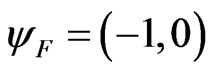 .
.
If the Certainty Degree is positive (DC > 0), then the Vector of State  will be on the lattice vertex which is the extreme Paraquantum logical state True:
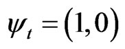 .
.
If the certainty degree is nil (DC = 0), then there is an undefined Paraquantum logical state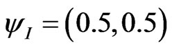 .
.
The module of a Vector of State  is:
is:
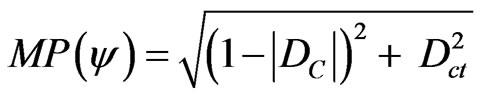 (6)
(6)
where: DC = Certainty Degree computed by (5);
Dct = Contradiction Degree computed by (4).
1) For DC > 0 the real Certainty Degree is computed by:
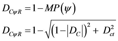 , (7)
, (7)
where: DCψR = real Certainty Degree.
2) For DC < 0, the real Certainty Degree is computed by:
 . (8)
. (8)
3) For DC = 0, then the real Certainty Degree is nil.
When the module of the Vector of State is of larger value than the unit MP(ψ) > 1, means that the Paraquantum logical state ψ are in an uncertainty region.
The intensity of the real Paraquantum logical state is computed by:
 . (9)
. (9)
When the superposed Paraquantum logical state ysup propagates on the lattice of the PQL a value of quantizetion for each equilibrium point is established [5,6,9]. This point is the value of the contradiction degree of the Paraquantum logical state of quantization (yhy ):
 , (10)
where: hy is the Paraquantum Factor of quantization.
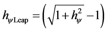
The factor hy quantifies the levels of energy through the equilibrium points where the Paraquantum logical state of quantization (yhy), defined by the limits of propagation throughout the uncertainty of the PQL, is located. Since the propagation exists, then we have to take into account the factor related to the Paraquantum Leaps which will be added to or subtracted from the Paraquantum Factor of quantization [5] such that:
 . (11)
In the language of the Paraquantum Logics, the entanglement between the favorable Evidence Degree (μ) and de unfavorable Evidence Degree (λ) produces the representation of a final Paraquantum logical state  visualized through the Intensity Degree of the Real Paraquantum logical state (μψR) (Equation (9)).
Figure 1 shows the effect of the Paraquantum Leap in the quantization of values when the Superposed Paraquantum Logical states (ysup) reach the point where the Paraquantum Logical state of Quantization (ψhψ) on the PQL Lattice. Where, from Figure 1 we can make the calculations:
 . (12)
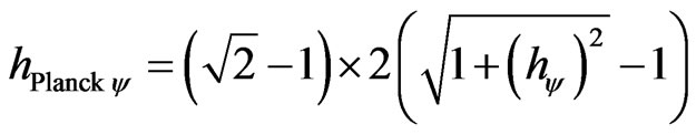
So, the Paraquantum Factor of quantization in its complete or total form which acts on the quantities is:
 . (13)
Comparisons and analogies between the International unit Systems and the British System result in a proportionality factor  related to the British system [10,11]. Therefore, in order to apply classical logics in the Paraquantum Logical model [6,9,11,12], the Newton Gamma Factor is
 .
.
In the paraquantum analysis [7] related to the series obtained from consecutively applying the Newton Gamma Factor  we define a correlation value called Paraquantum Gamma Factor
  such that:
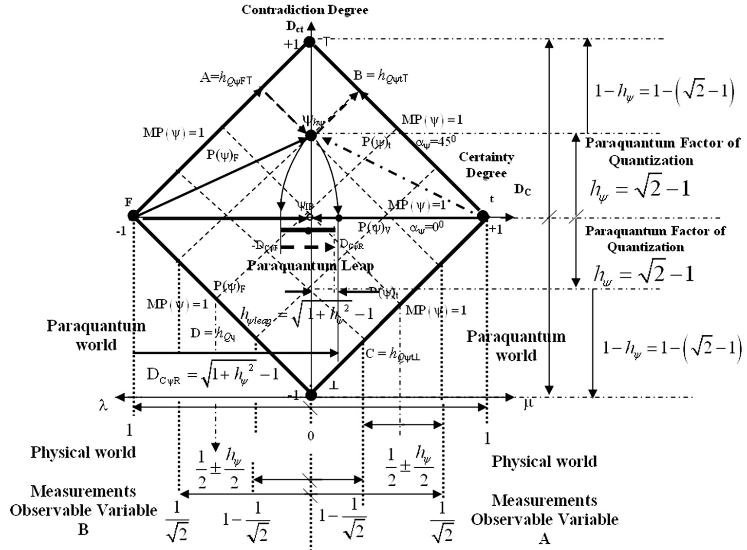
Figure 1. The paraquantum factor of quantization hy related to the evidence degrees obtained in the measurements of the observable variables in the physical world.
 , (14)
where:  is the Newton Gamma Factor:
 ,
,
 is the Lorentz factor which is:
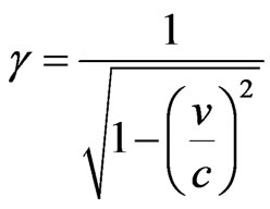 .
.
Using the Paraquantum Gamma Factor  allows the computations, which correlate values of Observable Variable in the physical world.
Evidence Degrees and the Time Calculations
In the paraquantum analysis the time has action directly in the measurements of the Observable Variables of the physical world. Considering the time as a Variable Observable the Equations (4) and (5) are now dependent of the time measurement, therefore:
 (15)
(15)
 . (16)
And the Paraquantum logical state (y):
 .
.
The variation of the time makes the values of the measurements in the Observable Variables modify and, as consequence, appear a propagation of the Paraquantum logical state through the PQL Lattice. At the referential of the Universe of Discourse [13] of the paraquantum analysis the favorable Evidence Degree of the Variable Observable time ( ) is:
) is:
 .
.
Considering the relativity theory concepts (seen in part I and [13]):
 . (17)
Similarly, we can write the equation of the unfavorable Evidence Degree depending on the Factor of Lorentz, which will be computed by the complement of the :
:
 . (18)
So, the greater the Factor of Lorentz  is, the closer to zero is the unfavorable Evidence Degree extracted from the Observable Variable time that is.
The Evidence degree values of the Observable Variable space/time and the Observable Variable velocity are in the Relativity theory [13], so, are dependent of the Lorentz factor. As, for these equations the velocity that is related to the speed of light in vacuum is equal to zero, then the Lorentz factor is unitary ( ). This causes the value of the Paraquantum Gamma Factor, which acts in these equations extracted in the Newtonian universe, is always the inverse of the factor of Newton:
 .
.
2. The Paraquantum Analysis in Newtonian Universe
As has been studied in part I of this work, for the paraquantum analysis of the Physical Systems in the Newtonian universe the space as Variable Observable, and the time as Variable Observable, are considered separately. In this way, the action of the Paraquantum Gamma Factor  is only in the Variable Observable of the time. In this case, the information source 1 presents the variation of the space is:
 .
.
And the information source 2 presents the variation of the time is: .
.
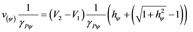
This manner, in the Newtonian universe the favorable Evidence Degree of Observable Variable velocity is extracted of two source of information.
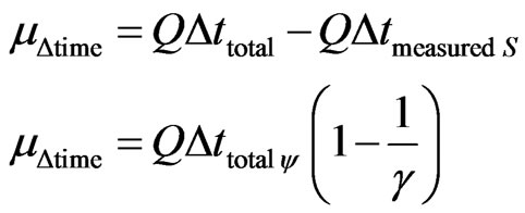
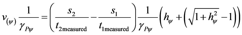
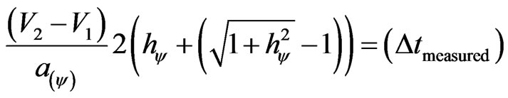
For the unitary value of the Discourse Universe (or Interest Interval), in the Newtonian universe the Paraquantum Gamma Factor acting in the time correlates in the equilibrium point the three greatness physics [9,12], such that:
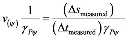 , (19)
where:
 = paraquantum velocity;
 = measured variation of time;
 = measured variation of space;
 = Paraquantum Gamma Factor by (14), were in Newtonian universe, is:
 .
.
The paraquantum velocity is the representation of the velocity of the body which is considered as a physical state of motion in the PQL because it is represented by a Paraquantum Logical state (ψ). For a type of static analysis, therefore without propagation of the Paraquantum logical state (ψ), the quantized paraquantum velocity in the equilibrium point is:
 , (20)
where: 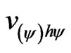 = paraquantum quantized velocity.
Figure 2 shows the representation of time (t) and space (s) and the result of the space-time paraquantum relation on the y-axis of the PQL Lattice with velocity.
According to the foundations of the PQL, the quantized paraquantum velocity in the equilibrium point is represented in the vertical y-axis of the contradiction Degrees.
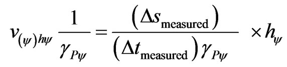
When the analysis is made for a dynamical process the Equation (20) of quantization velocity considers the Paraquantum Leap and becomes:
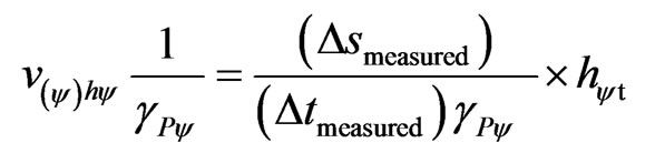 . (21)
From Equation (13): 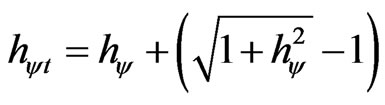 then:
then:
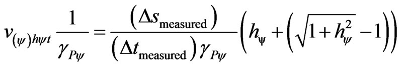 (22)
(22)
 .
.
From (19) we can rewrite (22) as follows:
 .
.
According to the physical laws, and using the previous equation, we can obtain the paraquantum acceleration in the Newtonian universe:
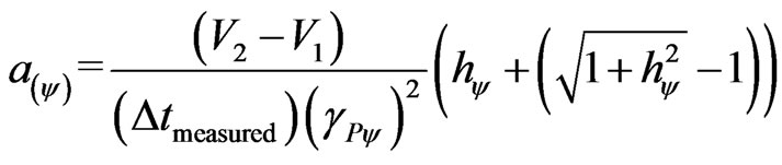 , (23)
where:
 = value of velocity measured at the start;
 = measured time variation;
 = quantized value of the state of acceleration of the system;
 = value of velocity measured at the end;
 = Paraquantum Gamma Factor (Equation (14));
 = measured of traveled space;
 = Paraquantum Factor of quantization.
Considering the equation that expressed Newton’s second law [10,11], we can isolate the Force F of the paraquantum analysis, such that:
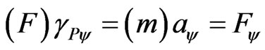 .
.
Being Force obtained by: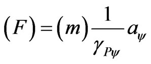 .
.
Using in this equation the expression of the paraquantum acceleration (23), we have:
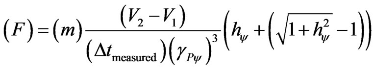 .
.
This last equation can be rewritten in such a way the one of the Observable Variables may be represented with
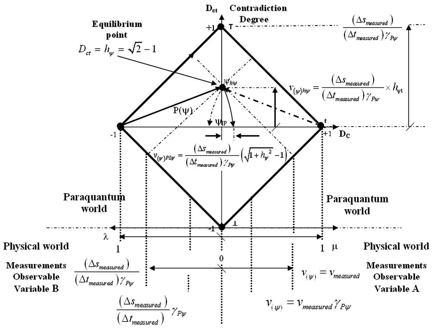
Figure 2. Representation of time (t) and space (s) and the result of the space-time paraquantum relation on the y-axis of the PQL Lattice with velocity.
quantized values by the action of the Paraquantum Gamma Factor, such that:
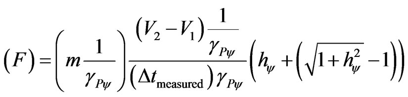 . (24)
Hence, for a value of Force F equal to the measured value, that is, without receiving the action of the Paraquantum Gamma Factor, we have:
1) the measured value of the variation of velocity  is multiplied by the inverse value of the Paraquantum Gamma Factor;
2) the measured value of time variation  is multiplied by the value of the Paraquantum Gamma Factor;
3) the value of the mass m of the body is multiplied by the inverse value of the Paraquantum Gamma Factor.
The value of the average velocity is already multiplied by the value corresponding to evidence Degree of Indefinition of the Paraquantum analysis. Hence, the average velocity in the Paraquantum Logical Model has a value computed according to the laws of physics [11] we have:
 →
→ . However, in the Newtonian universe, inverse value of the Newton Factor is considered, so the equation of average velocity can be expressed in a paraquantum form as follows:
 , (25)
where:
 = quantized value of average velocity which is equal to the value obtained by the laws of physics;
 = measured value of final velocity;
 = measured value of initial velocity;
 = Newton Gamma Factor which is
 .
.
The equation of traveled space can be written in a paraquantum fashion as follows:
 . (26)
From (23) that expresses the paraquantum acceleration and using the approximation of the Paraquantum Gamma Factor as being the inverse value of the Newton Factor, we have:
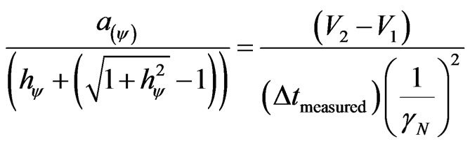 . (27)
Isolating V2 in Equation (27), we have:
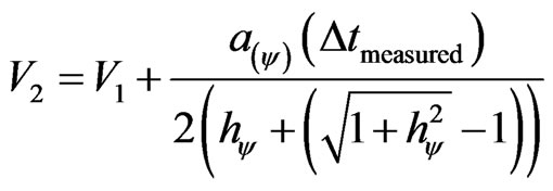 .
.
Replacing this value of V2 in (26) of traveled space ∆s, we have:
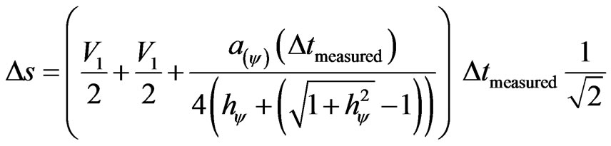 ,
,
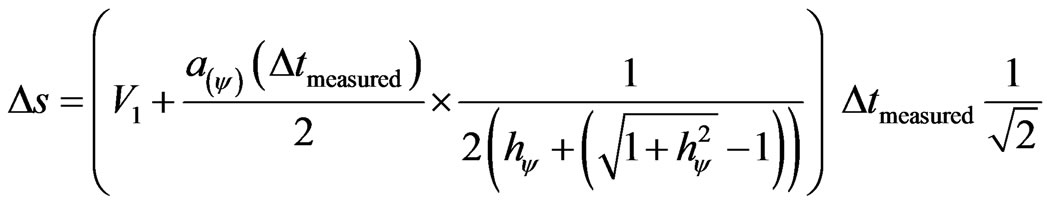 ,
,
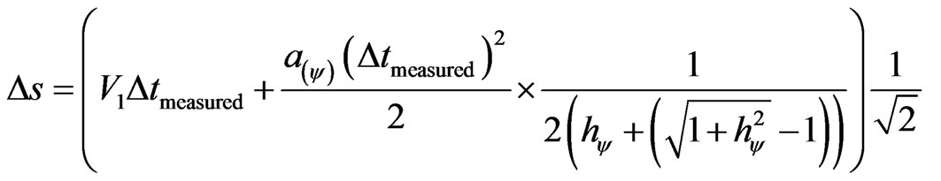 .
.
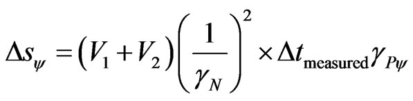
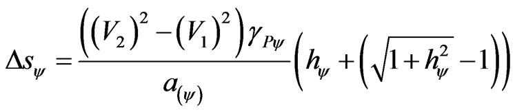
Going back to the value of the Paraquantum Gamma Factor, the equation of space which due to the use of paraquantum largenesses expresses a paraquantum value producing it by:
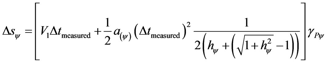 , (28)
where:
 = variation of space traveled obtained from paraquantum values;
 = measured value of initial velocity;
 = Paraquantum Gamma Factor;
 = measured variation of time;
 = value of acceleration of the body in study related to the paraquantum world;
 = Paraquantum Factor of quantization.
Isolating V1 in Equation (27), we can be written:

or:
 .
.
Which replaced in (28) produces:
 .
.
Going back to the value corresponding to the Paraquantum Gamma Factor in the Newtonian universe, we have:
 . (29)
When the Observable Variables that produce the Evidence Degrees are values of space traveled with square velocity, we can obtain the equation that determines the paraquantum acceleration:
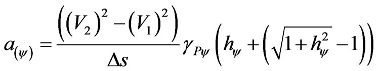 . (30)
Using Equation (30) of acceleration and equation which expresses Newton’s second law mathematically [10,11], Force can be computed by multiplying mass by the Paraquantum acceleration, such that:
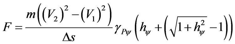 .
.
From the laws of classical physics [11] we obtain Work multiplying the value of Force by the displacement, then:
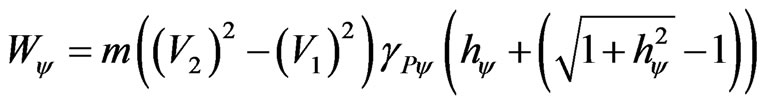 .
.
The paraquantum Work (Wψ) is identified with the total kinetic Energy at the equilibrium point where the Paraquantum Logical state is located: .
.
Therefore, the total kinetic Energy is expressed by:
 . (31)
And the equation of the paraquantum kinetic energy, represented at the equilibrium point of the PQL Lattice, is expressed by:
 , (32)
where:
 = is the kinetic energy quantized with respect to the physical world;
 = Mass of the body being considered.
The Work performed in the physical universe is identified with the quantity of paraquantum kinetic energy quantized with respect to the physical environment. Being the kinetic Energy the system’s energy variation [10, 11], then, from the previous equation we can obtain the paraquantum final energy such that:
 . (33)
 = Quantized initial kinetic energy;
 = value of the velocity measured at the start.
 , (34)
where:
 = Quantized final kinetic energy;
 = value of the velocity measured at the end.
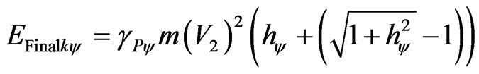
The total amount of energy involved in the Paraquantum Logical Model in a static state is that one computed at the value of the measured final velocity such that:
 . (35)
When related to the physical environment, the paraquantum total energy in the static state is expressed by:
 , (36)
where:
 = Total energy of the system involved by the Paraquantum Logical Model in the static state;
 = Total quantized Energy of the system involved by the Paraquantum Logical Model;
 = Final value of measured velocity.
As the analysis is done in the Newtonian Universe the velocity in these equations is not related to the speed of light in a vacuum c, but obtained by dividing the space and time, where only time suffers the action of Paraquantum Gamma Factor [10,13]. As, for these equations the velocity that is related to the speed of light in vacuum is equal to zero, then the Lorentz factor is unitary ( ). This causes the value of the Paraquantum Gamma Factor, which acts in these equations extracted in the Newtonian universe, is always the inverse of the factor of Newton:
 .
.
Figure 3 shows the representation of time (t), space (s) and of the mass (m) that is multiplying the velocity squared (V2). Is verified that for Newtonian universe the mass is constant and the total Paraquantum energy  is represented only in the y-axis of the PQL Lattice.
3. The Paraquantum Analysis and Fundamentals of an Unified Calculation
The equations of paraquantum velocity, acceleration, space, work and energy found in the Newtonian universe were extracted from Newton’s laws [10,11] and consider calculation always in equilibrium point located in the vertical y-axis of the PQL Lattice.
Comparing the amounts of total energy with the quantized pure final kinetic energy at the equilibrium point, we have:
 .
.
Being the quantized pure final kinetic energy obtained at the equilibrium point represented by:
 . (37)
Since the Paraquantum Logical Model is normalized, there is a complemented quantized pure kinetic energy, therefore, from Figure 3:
 . (38)
So, the total amount of total kinetic Energy, without adding the effect of the Paraquantum Leaps to it, appears as the unit on the axis of the contradiction degrees of the PQL Lattice, so that the normalized value is computed by:
 . (39)
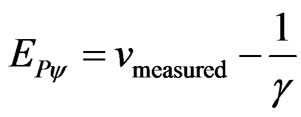
Equation (39) is for generalized values, however, for the relativity theory the pure complemented final kinetic energy can be written taking the unitary value in which it is bounded by the speed of the light c in the vacuum, such that:
 , (40)
where:
 = complemented final quantized kinetic Energy;
 = Constant value of the velocity of light in the vacuum, imposed as maximum value;
 = measured value of the particle’s velocity;
 = Mass of the particle being considered.
From Equation (40) we can write the paraquantum equation such that:
 . (41)
For this condition the PQL Lattice is bounded by the velocity c of light in the vacuum, such that now it is possible to obtain the paraquantum pure total energy based
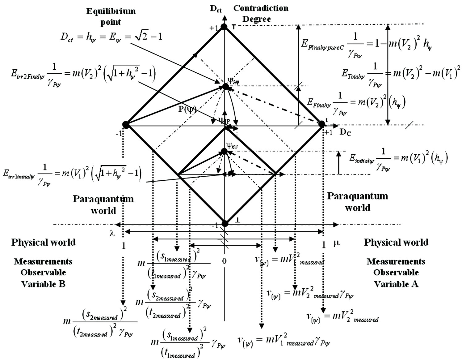
Figure 3. Representation of time (t), space (s) and of the mass (m) that is multiplying the velocity squared (V2)-with the paraquantum kinetic energy E(ψ) represented in the y-axis of the PQL lattice.
on the maximum bound which is the velocity of light in the vacuum. This is done by an equation of approximated values of the Equation (41) such that:
 , (42)
where:
 = Paraquantum pure total kinetic Energy of the system involved in the Paraquantum Logical Model;
 = Constant value of the velocity of light in the vacuum, imposed as maximum value;
 = Paraquantum Gamma Factor.
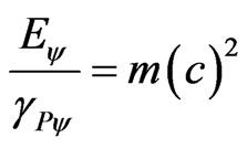
Which related to the physical environment it is expressed by:
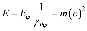 , (43)
where:
 = Pure total kinetic Energy of the system involved in the Paraquantum Logical Model;
 = Paraquantum pure total kinetic Energy of the system involved in the Paraquantum Logical Model.
3.1. Energy Calculations in Quantum Mechanics and Quantization Frequency
The propagation of the Paraquantum Logical state ψ on the Fundamental Lattice of the PQL depends on the frequency of the intensity variation or amplitude of the Observable Variables in the physical environment.
The Paraquantum Logical Model is applied in any form of variation of the physical quantities which are being considered as Observable Variables for the extraction of the Evidence Degrees μ or λ.
Figure 4 shows as an example a senoidal variation of the Evidence Degrees in the physical world which causes the propagation of the Paraquantum Logical state ψ represented by the Vector of State . We observe that the variation of the senoidal signal does not change the form of propagation of the Paraquantum Logical state ψ which continues propagating through infinitely many points established by infinitely local transition lattices.
3.1.1. Energy and Linear Momentum
In order to obtain the equations that express the energy related to the quantization frequency on the Paraquantum Logical Model, we initially consider a relation between the Momentum P and the Energy of the physical System being studied. Being the limits of the Lattice defined in this way, the paraquantum pure total energy determined by the quantization which exists on the Fundamental Lattice of the PQL has its value bounded by the velocity of light c in the vacuum [7,10,11].
Taking the relation from Equation (42):
 .
.
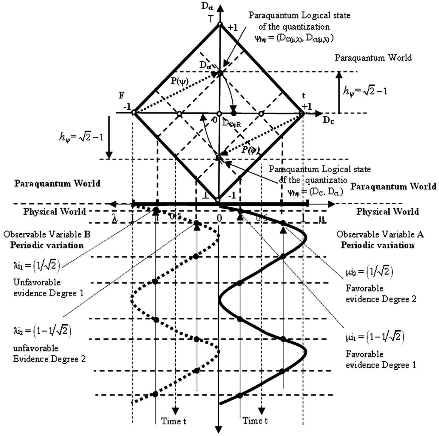
Figure 4. Senoidal variation of the evidence degrees in the physical world which causes the propagation of the paraquantum logical state ψ represented by the vector of state P(ψ).
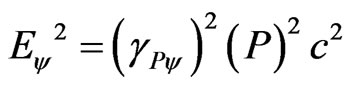
Squaring both sides of the previous equation and considering the linear Momentum P as being the product of mass m by velocity c, we have that:
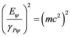 →
→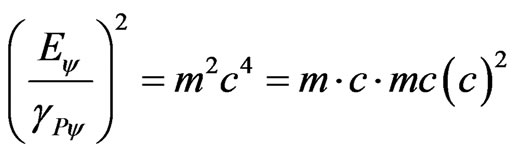 →
→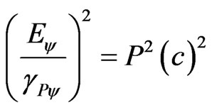 .
.
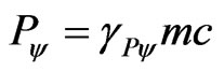
Being  the Paraquantum Momentum affected by the action of the Paraquantum Gamma Factor, such that:
 →
→ . Then:
 , (44)
where:
 = Paraquantum pure total Energy of the system involved by the Paraquantum Logical Model;
 = Momentum or quantity of linear movement.
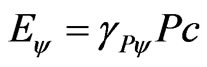
The equation of Energy at the physical environment and related to the Linear Momentum and to the velocity c of light:
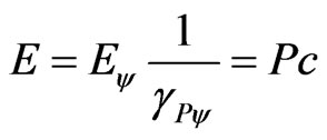 . (45)
The existence of the Paraquantum Gamma Factor on the equation points out that the fraction of velocity v of the body is related to the velocity c of light in the vacuum.
3.1.2. The Lattice of Inertial or Irradiant Energy
According to the paraquantum analysis, a fundamental Lattice of the PQL can receive the Evidence Degrees varying their intensity periodically because the Evidence Degrees are being extracted from quantities expressed by periodical functions, that can be of the type sin wt or cos wt. In this case, for the paraquantum analysis, it means a propagation of the Paraquantum Logical state ψ that makes the Vector of State  vary in module, such that in the variation the Paraquantum Leaps will produce inside the Fundamental Lattice a Lattice of Inertial or Irradiant Energy that will be expanding or contracting with frequency f.
3.1.3. Equation of the Inertial or Irradiant Energy and Frequency
Equation (12) expresses the energy of the Paraquantum Leap with the Inertial or Irradiant Energy  as being that one which varies when the Paraquantum Logical state ψ, in its propagation, passes by the equilibrium point of the Fundamental Lattice of the PQL. So, the variations of the Observable Variables in the physical environment generate inside the Fundamental Lattice of the PQL a Lattice of Inertial or Irradiant Energy that has the same properties of quantization of the Fundamental Lattice. Therefore, in the PQL Lattice of Inertial or Irradiant Energy the variation of emitted or absolved energy through the Paraquantum Leaps is proportional to the quantization frequency.
On the Paraquantum Logical Model, the value of the Inertial or Irradiant will be influenced by the action of the Paraquantum Factor of quantization  on its process of expansion and contraction. So, considering Bohr’s model:
If the maximum Energy exposed on the horizontal axis of the PQL Lattice of Inertial or Irradiant Energy is given by , then, in a complete orbit of the electron, the quantized Inertial or Irradiant Energy (
 ) will be computed by the application of the Paraquantum Factor of quantization. This condition is expressed by:
 , (46)
where:
 = Quantized Energy of the Lattice of Inertial or Irradiant Energy;
 = Maximum Energy of the Lattice of Inertial or Irradiant Energy obtained on the Fundamental Lattice;
 = Paraquantum Factor of quantization.
The multiplication by 2 is due to the analysis of a complete orbit on Bohr’s model.
3.1.4. The Paraquantum Planck Constant and Paraquantum Elementary Charge
From Equation (46) we can obtain, on the PQL Lattice of Inertial or Irradiant Energy, two important constants used on the equations that model phenomena of the Physical Systems. Being the Inertial or Irradiant Energy on the Fundamental Lattice computed by:
 , (47)
or by:
 , (48)
where: 
Considering the paraquantum Inertial or Irradiant Energy obtained from Equation (46): .
.
So, doing (48) in (46), this one is expressed by:
 . (49)
From Equation (49) we can determine:
1) The paraquantum Planck’s constant ( ) such that:
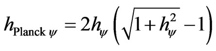 , (50)
2) The paraquantum elementary charge:
 . (51)
Since , then from Equation (51) we can determine the value of the paraquantum elementary charge of the electron which is:
 →
→ .
.
Therefore, as seen on Equation (50) the Paraquantum Factor of Quantization  and the paraquantum Planck’s constant
  are related by the paraquantum elementary charge such that:
 . (52)
Since , then from Equation (52) we can determine the value of the paraquantum Planck’s constant such that:
 →
→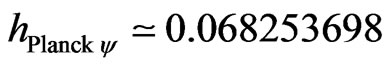 .
.
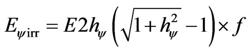
The Equation (46), which expresses the Paraquantum Inertial or Irradiant Energy, is written as follows:
 (53)
(53)
or:
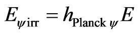 . (54)
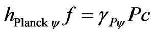
3.1.5. The Paraquantum Wavelength of De Broglie
Equation (49) deals with the Inertial or Irradiant Energy on the condition of two Paraquantum Leaps where the electron which orbits a core is an Observable Variable from where the Evidence Degrees, related to the electron’s position and momentum P for a complete lap, are extracted. For N orbits, we observe that the Inertial or Irradiant Energy is proportional to the frequency f which presents the Observable Variable in the physical world. So, taking into account the frequency of the Observable Variables, Equation (49) is presented with the values multiplied by the frequency such as:
or yet, from Equation (54), we obtain:
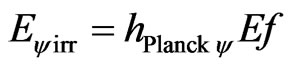 . (55)
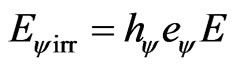
From Equation (55) we can consider that the paraquantum Planck’s constant multiplied by the frequency of the Observable Variable is a fraction of the quantization of the Inertial or Irradiant Energy of the Fundamental Paraquantum Logical Model. So, for the Paraquantum Logical Model we can express this fraction or quantizetion of the Inertial or Irradiant Energy, such as:
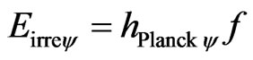 . (56)
where:
 = Quantization of the paraquantum Inertial or Irradiant Energy;
 = Frequency of the Observable Variable on the physical environment;
 = Paraquantum Planck’s constant such that
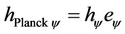 .
.
With:
 = Paraquantum Factor of quantization;
 = Paraquantum elementary charge:
 .
.
From Equation (56) we can isolate frequency, such that:
 .
.
The Observable Variables on the physical environment vary periodically in a senoidal way and in this condition, we can consider the fact that the distance between values repeated in a standard of a wave is called wavelength, represented by the Greek letter  [11,12]. For the Observable Variable on the physical environment, the wavelength can be determined by the wave velocity divided by its frequency such that:
 .
.
If it is an electromagnetic wave which travels in the vacuum, its velocity is the same value of the velocity c of light in the vacuum, therefore, the wavelength can be expressed by:  or represented by frequency, such that:
 .
.
Then: , were we can isolate wavelength:
 . (57)
Since frequency is obtained through the wavelength and the velocity of the particle, we can consider that Equation (56) expresses its linear Momentum P such that the equalities are valid: 
 (58)
(58)
or yet:
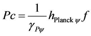 . (59)
Since wavelength  relates inversely with frequency f, we have that:
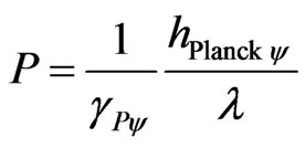 . (60)
So, we can find the wavelength of De Broglie [10,12] in the paraquantum analysis such that:
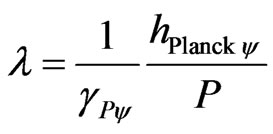 . (61)
The representation of stationary wave, which is linked to the electron orbit of radius r around the core, is compared to a string attached to the edges [11]. The natural ways of vibration of a string of length d with one end attached means that in each end there is a knot. This means that the wavelength  must be chosen such that:
 with
with  Therefore:
 .
.
For a wavelength  considered as the wave of a circular orbit of the electron, such that comparing with the vibrating string, we have:
  →
→ .
.
Since Momentum is given by: .
.
Then by Equation (61) we have: .
.
Doing:  we have:
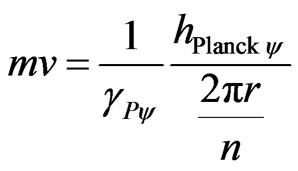 →
→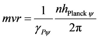 .
.
The radius of the orbit of the electron is given by:
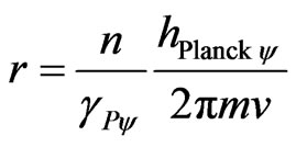 . (62)
Since, from Equation (52): .
.
We can relate the paraquantum values in a way that the radius of the orbit of the electron is computed by:
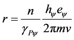 . (63)
The number n of times that a quantization happens, therefore, the number of times that the Paraquantum logical state ψ passes by the equilibrium point is proportional to two times the energy produced by the Paraquantum Leap.
Considering the analysis on the Fundamental Lattice of the PQL applied on an orbital model of an electron around a core, as the study which deals with Bohr’s model, Paraquantum Leaps will happen on the equilibrium point in each variation period [14,15]. With the results of study of Paraquantum Logical Model of hydrogen atom shown in [14] and [15] we can verify the values related to quantization factors and the equilibrium point.
3.1.6. Energy Calculations in Hydrogen Atom by Paraquantum Analysis
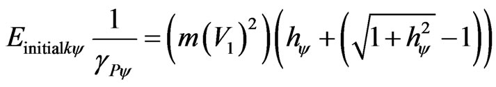
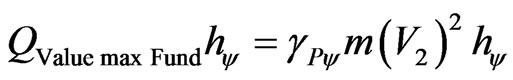
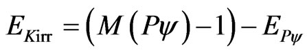
As was shown in [14,15] we can use the Paraquantum logical model to calculate energy levels in hydrogen atom. Comparing the amounts of total energy with the quantized pure final kinetic energy at the equilibrium point the equation of the quantities of Energy, for the Bohr’s model on the Hydrogen atom, can be written as follows:
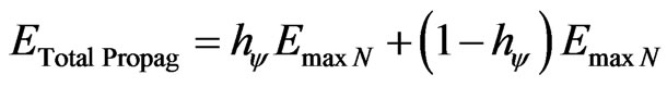 , (64)
where: hψ is the Paraquantum Factor of quantization.
 is the total Energy that can be transformed through propagation, therefore through the orbit of the electron in the Hydrogen atom.
 is the maximum energy on the level N of transition frequency or in the current state of excitation of the electron.
N is the transition frequency or number of times of application of the Paraquantum Factor of quantization.
The value of the quantity of Energy of Propagation quantized, when considered in its static form, therefore, without considering the effect of the Paraquantum Leap, is computed by:
 . (65)
Since the process of transformation of energy is dynamical, we must consider the effects of Paraquantum Leaps on the Paraquantum Logical Model. So, the Inertial or Irradiating Energy is expressed by:
 . (66)
The total energy transformed at the equilibrium point of the Lattice of the PQL is computed by:
 . (67)
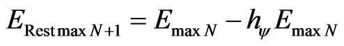
So, Equation (64) is rewritten as follows:
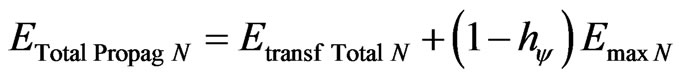 , (68)
or as follows:
 . (69)
Or, in a more complete way, as follows:
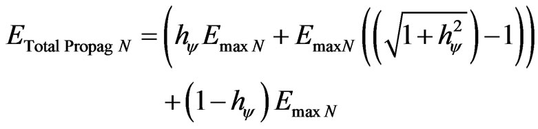 . (70)
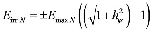
The second term of Equation (69) is the complemented value which represents the remaining maximum energy, therefore, it is that amount of energy capable of still being transformed in order to increase the excitation level of the electron. So, for each new excitation level of the electron, the remaining energy ERest max is the one which outcomes the value which will be represented on the vertical and horizontal axis of the Lattice of the PQL. For a static analysis, we have:
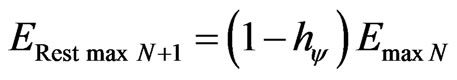 (71)
(71)
or
 . (72)
From (72) the energy variation value is expressed by:
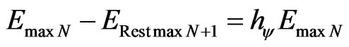 . (73)
Therefore, the remaining maximum Energy in the atom model depends on the excitation level of the electron.
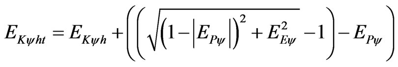
When the analysis process is considered dynamical, we must take the effect of the Paraquantum Leap into account and determine the Remaining maximum Energy adding the Inertial or Irradiating Energy. So, Equation (72) in its complete form is:
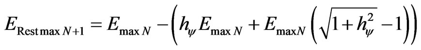 .(74)
.(74)
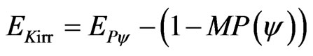
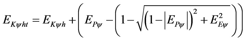
And the energy transformed value between the Fundamental level n = 1 and the level N = n is:
 . (75)
A Paraquantum Logical model used in analyses of quantum mechanics environments produce a contraction effects in the PQL Lattice [9,14,15].
Figure 5 shows Paraquantum Logical Model in analyses of Hydrogen atom with the contraction effects at Lattices.
3.2. Energy Calculations in Relativity Theory Universe by Paraquantum Analysis
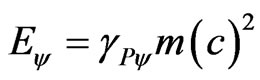
As was seen in part I of this work, the Equations (40)-(43) are only valid in the universe of the theory of relativity at the equilibrium point, where the Lorentz Factor and the Paraquantum Gamma Factor are equal, such that:  The correlation of the equilibrium point of the Theory Relativity PQL Lattice and PQL Lattice
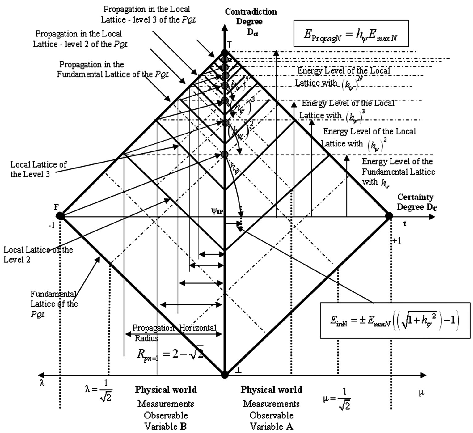
Figure 5. The paraquantum logical model in analyses of quantum mechanics with the contraction effects at lattices.
of the Newtonian universe indicates a relation:
For Theory Relativity PQL Lattice →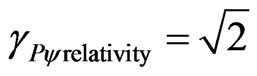 ;
;
For Newtonian universe PQL Lattice →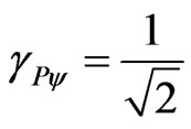 ,
,
 .
.
Considering a gradual increase from zero of the velocity (v) relative to the speed of light in vacuum c is verified that the Paraquantum logical State (ψ) moves as increases the value of the Lorentz Factor. In this case, as the Paraquantum logical state (ψ) is out of equilibrium point, the calculations have to consider so many values exposed on the y-axis, the degrees of contradiction, as well as the values for the x-axis, of the certainty degrees.
The equations of the degree of contradiction represent the kinetic energy, which in a dynamic analysis has added energy inertial or irradiant from Paraquantum leap.
Following this same procedure, now with the Paraquantum logical state (ψ) outside of the equilibrium point, on the x-axis the values of the Potential Energy will be exposed. It is verified that in the Relativity Theory the values of the Potential Energy are linked to effects of increase of the mass.
Figure 6 shows a representation of PQL Lattices to correlate the areas of Science Physics, where the energies may be represented and studied on the axes.
When the Paraquantum logical State (ψ) moves to the extreme point of the vertex right of the Lattice the value of the inertial energy (or irradiant) added to the kinetic energy decreases. There will also be a decrease in kinetic energy (Degree of contradiction—y-axis) and an increase in potential energy (Degrees of certainty—x-axis).
From Equation (16): 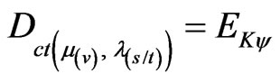 with
with  and
and :
:
 (76)
(76)
 = Pure total kinetic Energy.
And from Equation (15): 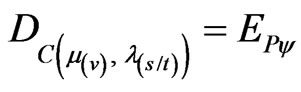
 (77)
(77)
 = Potential Energy.
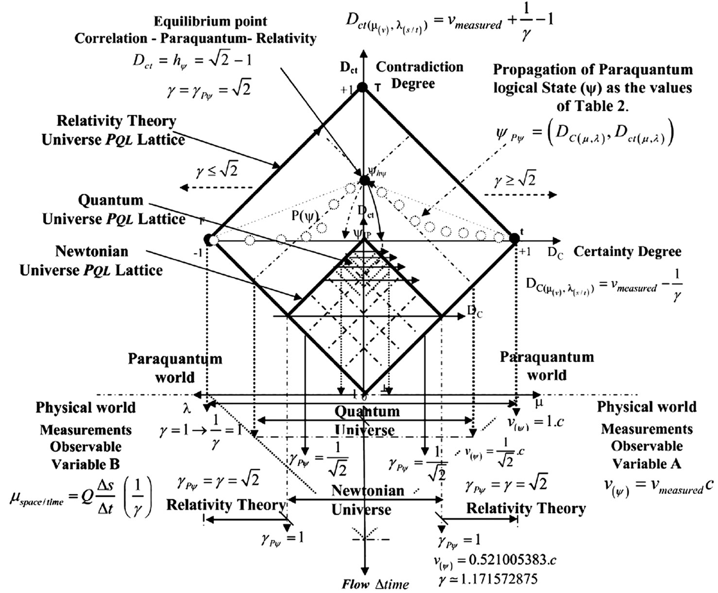
Figure 6. Representation PQL lattices to correlate the areas of science physics.
In the equilibrium point with: ,
,
 and
and .
.
From Equation (76):
 = Pure quantized kinetic Energy.
And from Equation (77): 
Out of the equilibrium point the total kinetic Energy is:
 .
.
Were the inertial energy (or irradiant)  is computed as follows: If
 →
→ .
.
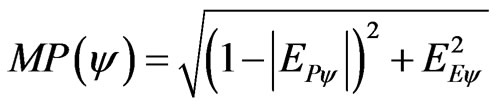
Being  the module of a Vector of State
  obtained by Equation (6), that with represented energy is:
 .
.
Therefore the total kinetic Energy for Relativity theory universe is:
 , (78)
If  →
→ ,
,
 . (79)
When the velocity v relative to the speed of light in a vacuum c approaches the unit, then the Paraquantum logical State (ψ) approaches the vertex far right Lattice.
At this point the sum of kinetic Energy ( ) with Inertial Energy (or irradiant) (
 ) results in value around zero (
 ) and the Potential Energy is maximal with value close to unity (
 ).
).
In this extreme condition the space-time construct has value close to zero ( ) and the value of the mass effect is close to the unit.
Table 1 shows the values of the Lorentz Factor and Paraquantum Gamma Factor and variations produced in degrees of evidence of paraquantum analysis applied to the Relativity Theory.
Figure 7 shows the representation of space-time and of the velocity v related at speed of the light in the vacuum c. The Paraquantum kinetic energy  is in the y-axis and the Paraquantum Potential energy
  is in the x-axis of the PQL-Relativistic Lattice.
3.3. Discussion
The effects related to energy in the Newtonian universe, in the universe of the theory of relativity and in quantum mechanics, can be represented in a single Lattice of the
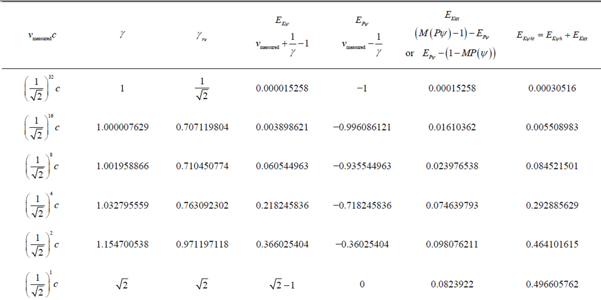
Table 1. Results of the energy values for diferent velocity values in the paraquantum relativity equations.
Paraquantum logic. The maximum PQL Lattice is the Paraquantum/Relativity, as seem in Figures 6 and 7, and some characteristics of paraquantum analysis can be listed as:
For PQL Lattice in Quantum Mechanics → .
.
• The Paraquantum Gamma Factor is fixed;
• Quantization of the kinetic energy is made through of the Paraquantum Factor of quantization (hψ);
• There is an irradiant Energy (or Inertial) due to Paraquantum leaps;
• Quantization is made through the equilibrium points of lattices that are contracted;
• For higher level of quantization the degree of certainty will be smaller.
For PQL Lattice in Newtonian World →  .
.
• The Paraquantum Gamma Factor is fixed;
• Quantization of the kinetic energy through of the
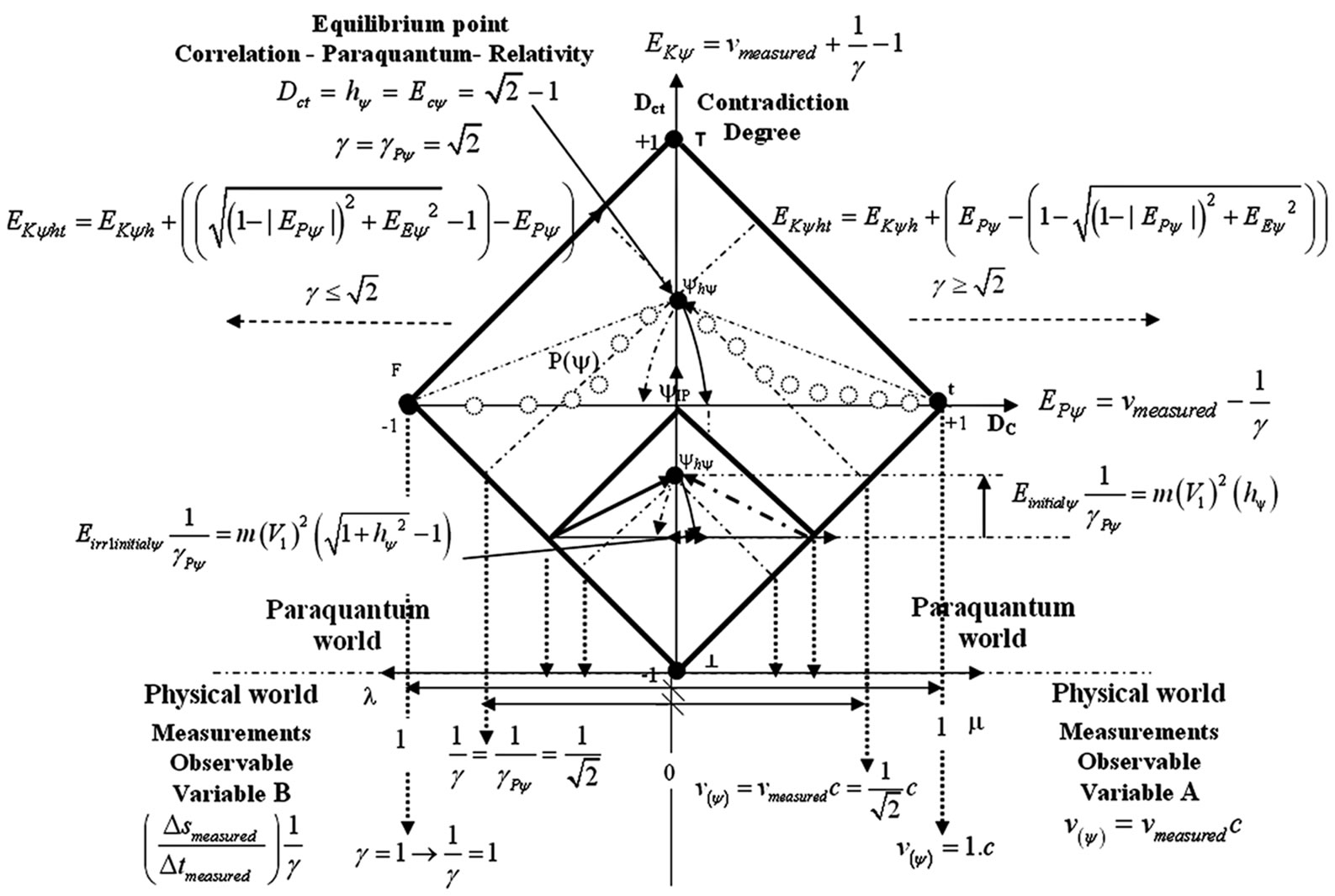
Figure 7. Representation of space-time and of the velocity v related at speed of the light in the vacuum cwith the paraquantum kinetic energy Ec(ψ) in the y-axis and the paraquantum Potential energy Ep(ψ) in the x-axis of the PQL-Relativistic lattice.
Paraquantum Factor of quantization (hψ) related at variation in evidence degrees;
• There is an irradiant Energy (or Inertial) due to Paraquantum leaps;
• Quantization is made through the equilibrium points of lattices that are expanded;
• For higher level of quantization the degree of certainty will be higher.
For PQL Lattice in Relativity World →  .
.
• The Paraquantum Gamma Factor is fixed only in the equilibrium point;
• Quantization of the kinetic energy through of the Paraquantum Factor of quantization (hψ) is made only in the equilibrium point;
• Quantization of the kinetic energy and of the Potential energy are made through of the Lorentz Factor;
• There is an irradiant (or Inertial) Energy due to Paraquantum leaps;
• The Lattice boundaries are fixed by the value of the speed c of light in a vacuum;
• For higher level of quantization the degree of certainty will be higher and the degree of contradiction is smaller.
4. Conclusions
In this paper we presented a study of physical phenomena that correlates the concepts of the Theory of the Relativity and foundations of the Paraquantum logic.
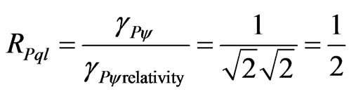
Through the originated Equations of the Paraquantum Logical Model we did analogies with relativistic effects where we verified the relation between the Factor of Lorentz γ and the Paraquantum Gamma Factor γPψ.
The effects of these factors were studied in detail and we observed that the Paraquantum Gamma Factor (γPψ)- which aggregates the phenomena found in the theory of relativity and in the Newtonian universe, makes the connection among the physical universes through the correlation with the Factor of Paraquantum Quantization hψ. This correlation produced equations about physical quantities where through the paraquantum equations we investigated the effects of energy balancing and quantization properties. With the paraquantum equations, in which the Paraquantum factors appear and deal with the Observable Variables as periodical variations, relation between quantizations and intensity frequencies of physical quantities were established. From these relations some important constants related to the studies of De Broglie appeared. So, with the interpretations on the PQL Lattice is possible to connect the values of the main constants of physics with the factors determined in the studies of the Paraquantum Logics. As demonstrated in this work, the results are easy to view through of the PQL lattices and shows with clarity the behavior of physical quantities in three main areas of study of physical science. Therefore, by all indications, the analysis through the Paraquantum Logic presents great possibilities to produce the fundamentals necessary for a unified physical theory.
REFERENCES
- N. C. A. Da Costa and D. Marconi, “An Overview of Paraconsistent Logic in the 80’s,” The Journal of NonClassical Logic, Vol. 6, No. 1, 1989, pp. 5-31.
- N. C. A. Da Costa, “On the Theory of Inconsistent Formal Systems,” Notre Dame Journal of Formal Logic, Vol. 15, No. 4, 1974, pp. 497-510. doi:10.1305/ndjfl/1093891487
- S. Jas’kowski, “Propositional Calculus for Contradictory Deductive Systems,” Studia Logica, Vol. 24, No. 1, 1969, pp. 143-157. doi:10.1007/BF02134311
- J. I. Da Silva Filho, G. Lambert-Torres and J. M. Abe “Uncertainty Treatment Using Paraconsistent Logic—Introducing Paraconsistent Artificial Neural Networks,” IOS Press, Amsterdam, 2010.
- J. I. Da Silva Filho, “Paraconsistent Annotated Logic in analysis of Physical Systems: Introducing the Paraquantum Factor of quantization hψ,” Journal of Modern Physics, Vol. 2, No. 11, 2011, pp. 1397-1409.
- D. Krause and O. Bueno, “Scientific Theories, Models, and the Semantic Approach,” Principia, Vol. 11, No. 2, 2007, pp. 187-201.
- J. I. Da Silva Filho, “Analysis of Physical Systems with Paraconsistent Annotated Logic: Introducing the Paraquantum Gamma Factor γψ,” Journal of Modern Physics, Vol. 2, No. 12, 2011, pp. 1455-1469.
- C. A. Fuchs and A. Peres, “Quantum Theory Needs no ‘Interpretation’,” Physics Today, Vol. 53, No. 3, 2000, pp. 70-71. doi:10.1063/1.883004
- J. I. Da Silva Filho, “Study of the Interactions between Particles Based in Paraquantum Logic,” Journal of Modern Physics, Vol. 3, No. 5, 2012, pp. 362-376. doi:10.4236/jmp.2012.35051
- Pl. A. Tipler and R. A. Llewellyn, “Modern Physics,” 5th Edition, W. H. Freeman and Company, New York, 2007.
- J. P. Mckelvey and H. Grotch, “Physics for Science and Engineering,” Harper and Row Publisher Inc, New York, London, 1978.
- Pl. A. Tipler, “Physics,” Worth Publishers Inc, New York, 1976.
- A. Einstein, “Relativity the Special and the General Theory,” Methuen & Co. Ltd., London, 1955.
- J. I. Da Silva Filho, “Analysis of the Spectral Line Emissions of the Hydrogen Atom with Paraquantum,” Journal of Modern Physics, Vol. 3, 2012, pp. 233-254.
- J. I. Da Silva Filho, “An Introductory Study of the Hydrogen Atom with Paraquantum Logic,” Journal of Modern Physics, Vol. 3, No. 4, 2012, pp. 312-333.