Applied Mathematics
Vol.07 No.14(2016), Article ID:70082,10 pages
10.4236/am.2016.714137
Zero Truncated Bivariate Poisson Model: Marginal-Conditional Modeling Approach with an Application to Traffic Accident Data
Rafiqul I. Chowdhury1, M. Ataharul Islam2
1ISRT, University of Dhaka, Dhaka, Bangladesh
2Department of Applied Statistics, East West University, Dhaka, Bangladesh

Copyright © 2016 by authors and Scientific Research Publishing Inc.
This work is licensed under the Creative Commons Attribution International License (CC BY).
http://creativecommons.org/licenses/by/4.0/


Received 25 June 2016; accepted 22 August 2016; published 25 August 2016
ABSTRACT
A new covariate dependent zero-truncated bivariate Poisson model is proposed in this paper employing generalized linear model. A marginal-conditional approach is used to show the bivariate model. The proposed model with estimation procedure and tests for goodness-of-fit and under (or over) dispersion are shown and applied to road safety data. Two correlated outcome variables considered in this study are number of cars involved in an accident and number of casualties for given number of cars.
Keywords:
Bivariate Poisson, Conditional Model, Generalized Linear Model, Marginal Model, Road Safety Data, Zero-Truncated

1. Introduction
The count data analysis occupies an important role in applied statistics in various fields. When the observed outcomes are count and the desire is to estimate the covariate effects on outcomes, covariate dependent Bivariate Poisson (BVP) model is a tool of natural choice. It is expected that the observed outcomes on the same subject are be correlated. This type of data arises in many fields, for example, traffic accidents, health sciences, economics, social sciences, environmental studies among others. A typical example of such dependence arises in the number of traffic accidents and the number of injuries or fatalities during a specified period. However, in some situations outcomes may be truncated as zero values of counts may not be observed or may be missing for one or both of the outcomes. For example, in a sample drawn from hospital admission records, frequencies of zero accidents and length of stay are not available. Another example is the case where the data on number of traffic accidents and related injuries or fatalities and related risk factors are collected from records and, naturally, zero counts are not available. As an example, road safety data from data.gov.uk website provides detailed information about the conditions of personal injury road accidents in Great Britain including the types of vehicles involved and the consequential casualties on public roads along with other background information. Only those accidents that involve personal injury reported to the police using the accident reporting form are recorded. Damage-only accidents, with no human casualties or accidents on private roads or car parks, are not included generating zero-truncated count data. To investigate the effect of risk factors on this type of outcomes, zero- truncated BVP regression is the appropriate model.
Campbell [1] introduced BVP distribution. Various assumptions have been used to develop BVP distribution. The most comprehensive one has been proposed by Kocherlakota and Kocherlakota [2] . Leiter and Hamdan [3] suggested bivariate probability models applicable to traffic accidents and fatalities. A similar problem was addressed by Cacoullos and Papageorgiou [4] . Several other attempts were made to define and study the BVP distribution [5] - [9] . Jung and Winkelmann [10] showed bivariate Poisson form using a trivariate reduction method allowing for correlation between the variables, which is considered as a nuisance parameter. This bivariate Poisson regression is used by others [11] [12] . Islam and Chowdhury [13] suggested covariate dependent BVP model using generalized linear modeling approach based on Leiter and Hamdan [3] bivariate probability models. They used marginal and conditional models to obtain BVP model.
Studies on the covariate dependent zero-truncated BVP model are scarce. Different techniques of the parameter estimation of BVP distribution are presented in [14] - [16] . A unified treatment of three types of zero-truncated BVP discrete distribution based on probability generating function is shown elsewhere [17] . Properties of BVP distribution truncated from below at an arbitrary point were studied by others [18] [19] . At this backdrop, we proposed a zero-truncated covariate dependent BVP model based on the work of Islam and Chowdhury [13] . The exposition of the following sections of the paper is as follows. Firstly in Section 2, we present briefly the marginal, conditional and BVP distribution for two outcomes without zero truncation as shown in [13] . In Section 3, we have shown the zero-truncated marginal and conditional Poisson distribution and obtained the joint model for both outcomes zero-truncated. The estimation and the related procedures are also shown. In Section 4, applications of the proposed models are illustrated using road safety data for both outcomes zero-truncated published by the Department for Transport, United Kingdom. Finally, concluding remarks can be found in Section 5.
2. Poisson Distribution without Zero Truncation
In this section bivariate Poisson model without zero truncation is shown. For simplicity, we shall follow the notations used in [13] . Let Y1 be the number of accidents at a specific location in a given interval that has a Poisson distribution with density
 (1)
(1)
and the corresponding link function is

If ’s are assumed to be mutually independent, then the conditional distribution of
  the total number of fatalities recorded among the Y1 accidents occurring in the jt-h time interval is Poisson with parameter
 . Then we can show that
 (2)
(2)
and the corresponding link function is

Then following [13] the joint distribution of number of accidents and number of fatalities can be shown as
 (3)
(3)
3. Zero-Truncated Poisson Distribution
The probability of  is
is , using Equation (1). Hence Y1 is observed conditional on Y1 > 0. Thus, we have the conditional probability mass function
 (4)
(4)
Now, using Equation (1) the zero-truncated Poisson probability mass function for  is
is
 (5)
(5)
Then the exponential form of the mass function is
 (6)
(6)
The mean and variance can be shown as
 (7)
(7)
Similarly, the zero-truncated conditional distribution of  is
is
 (8)
(8)
Then the zero-truncated conditional Poisson distribution is
 (9)
(9)
The exponential form of Equation (9) can be shown as
 (10)
(10)
Then the mean and variance are
 (11)
(11)
3.1. Zero Truncated Bivariate Poisson (ZTBVP) Model
Now using the marginal and conditional distribution for zero truncation derived above the joint distribution of ZTBVP can be obtained as follows
 (12)
(12)
The ZTBVP expression in Equation (12) can be expressed in bivariate exponential form as
 (13)
(13)
where the link functions are  and
and 
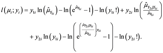
The log-likelihood function is
 (14)
(14)
The estimating equations are
 (15)
(15)
and
 (16)
(16)
Then the score vector is
 (17)
(17)
The second derivatives are:
 (18)
(18)
 (19)
(19)
The observed information matrix is
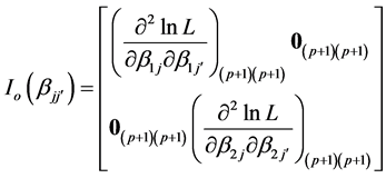 (20)
(20)
and the approximate variance-covariance matrix for  is
is  The estimates of the regression parameters vectors
  and
and  can be obtained iteratively by using Newton-Raphson method as follows
 (21)
(21)
where  denotes the estimate at t-th iteration.
3.2. Test for Significance of Parameters
We can use the likelihood ratio tests for testing  and
and  model fit using full model and reduced model. The test statistic is asymptotically chi-square as follows
 (22)
(22)
For independence, we can test the equality of zero-truncated bivariate models under independence. The independence model can be shown as .
.
3.3. Deviance and Goodness of Fit
The deviance measures the difference in log-likelihood based on observed and fitted values. Let  and
and  are the estimates of
  and
and  under the model of interest as shown before (Section 3.1) and
  and
and  are the observed values under the saturated model. The deviance for zero-truncated bivariate Poisson,
 , where
  represents log-likelihood functions, as follows:
 (23)
(23)
and
 (24)
(24)
After some algebra we get the deviance as
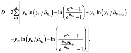 (25)
(25)
We can use following test for goodness-of-fit proposed by Islam and Chowdhury (2015).
 (26)
(26)
where,  are estimates of
  and
and ,
,  and
and  are estimates of
  and
and  as defined in Equations (7) and (11), respectively.
  is distributed asymptotically as
  where g is the number of groups of observed values,
 .
.
3.4. Test for Over or Underdispersion
The presence of overdispersion or underdispersion may influence the standard error of parameter estimates, hence, the significance level of the estimates. Test for the goodness of fit as shown in Equation (26) is modified to test the overdispersion or underdispersion. The method of moments estimator suggested by [20] is used to estimate the dispersion parameter,  , as shown below
 (27)
(27)
Using the mean, variance and correction factor as shown in [21] for truncated marginal and conditional Poisson models for  we can define
  and
and  where
where
 ,
,  ,
,  ,
, 
and then using these values we can estimate .
.
Then the test for dispersion  for zero-truncated bivariate Poisson regression model is:
 (28)
(28)
where,  are estimates of expected values and variances as defined in Equations (7) and (11) and
  and
and  are dispersion parameters for Y1 and Y2, respectively. T2, is also, distributed asymptotically as
  where g is the number of groups of observed values,
 .
.
4. Application
The models proposed in the paper are illustrated using the road safety data published by Department for Transport, United Kingdom. This data set is publicly available for download from UK givernment website (http://data.gov.uk/dataset/road-accidents-safety-data). The data set includes information about the conditions of personal injury road accidents in Great Britain and the consequential casualties on public roads. Background information about vehicle types, location, road conditions, drivers demographics are also available among others. A total of 1,494,275 accident records were in the data set spanning from 2005 to 2013. We have selected a random sample 14005 accident records approximately 1 percent of all accident records. The outcome variables considered are total number of vehicles involved in the accident (Y1) and the number of casualties (Y2). Due to small frequencies, values five or more were coded as five for both outcomes. Risk factors are sex of the driver (0 = female; 1 = male), area (0 = urban; 1 = rural), two dummy variables for accident severity (fatal severity = 1, else 0; serious severity = 1, else = 0; slight severity is the reference category), light condition (daylight = 1; others = 0) and eight dummy variables for year 2006 to year 2013, where year 2005 is considered as reference category.
The average number of vehicles involved in accident and casualties are 1.83 and 1.37, with standard deviations 0.75 and 0.92, respectively. Table 1 displays the bivariate distribution of the number of vehicles and number of casualties. It is evident that 59 percent of the accidents involved two cars, 30 percent single car, and eight percent three cars. The number of casualties was one in three-fourth of the cases and two in one out of six cases. Descriptive statistics of the number of vehicles involved in accidents and number of casualties by risk factors are presented in Table 2. The mean number of vehicles with fatal injuries was 1.94 compared to 1.70 and 1.85 with serious and slight injuries. The mean number of casualties was 2.15 for fatal cases which appears to be much higher than that of serious and slight injuries. There is not much variation in mean number of vehicles and casualties by sex of driver and area. Although the number of vehicles involved in the accident is higher during daylight, number of casualties appear to be higher during other times. The number of vehicles involved in accidents decreased steadily during the study period, but mean number of cars involved in accidents and casualties remained almost similar.

Table 1. Number of vehicles involved in the accident (Y1) and number of casualties (Y2).
We observe that both numbers of vehicles involved in accidents and number of casualties are heavily under- dispersed as displayed in Table 4. In Table 3, the estimates of the parameters are displayed along with standard errors and p-values for both original models as well as for adjustments made for underdispersion. Summary measures of goodness of fit for all the models are summarized in Table 4. The proposed full model of ZTBVP (Table 3) shows a negative association between fatal and serious severity and number of cars involved in accidents, while there is a positive association (p-value < 0.01) between the number of cars involved in an accident and light condition (daytime driving). The number of cars involved in accidents appears to be negatively associated in years 2008-2010 and 2012 as compared to that of 2005. However, the conditional model for the number of casualties given the number of cars involved in an accidents reveals that male drivers compared to females, rural areas compared to urban and daytime compared to night have lower risks. On the other hand, fatal severity and serious severity are positively associated with the number of casualties for given number of accidents compared to light severity. It is also evident that compared to the reference year, 2005, the number of casualties is negatively associated with the years 2012 and 2013. This indicates a significant reduction in the number of casualties for given number of accidents in recent years as compared to that of 2005.
Table 2. Descriptive statistics of the number of vehicles involved in the accident and the number of casualties by risk factors.
Table 3. Parameter estimates of zero truncated BVP model.
The summary results of estimation and tests of different models (proposed model based on marginal-condi- tional approach and both marginal models) are presented in Table 4. Both the full model and the reduced model under null hypothesis are considered. Both the models indicate that the full models are statistically significant. It is noteworthy that both the outcome variables number of vehicles involved in accidents and number of casualties are substantially underdispersed and adjustments were made accordingly for underdispersion in Table 3. Based on AIC, BIC and deviance we observe that the proposed full model using marginal-conditional approach provides the best fit. The goodness of fit test using the test statistic, T1, indicates good fit marginally (p-value = 0.064) for the proposed model. The test for under dispersion reveals the presence of significant deviation from equidispersion in both the variables as observed from T2 (p-value < 0.001). Adjustments are made for under- dispersion and the results are shown in Table 3 (last two columns).
Table 4. Test statistics results for reduced and full models of ZTBVP.
5. Conclusion
A zero-truncated bivariate generalized linear model for count data is proposed in this paper. This model is based on the bivariate model using marginal-conditional models proposed by Islam and Chowdhury (2015) for count data. Covariate dependent bivariate generalized linear model is shown, and canonical link functions are used to estimate the parameters of the Poisson distribution. The usefulness of the proposed model is demonstrated using road safety data published by Department for Transport, United Kingdom. The proposed ZTBVP model can easily accommodate a varying number of covariates for two outcomes. The joint distribution degenerates into a marginal and conditional distribution that makes estimation problem easier.
Acknowledgements
We acknowledge gratefully that the study is supported by the HEQEP sub-project 3293, University Grants Commission of Bangladesh and the World Bank. This data set was obtained from Police reported road accident statistics (STATS19) Department for Transport (http://data.gov.uk/dataset/road-accidents-safety-data).
Cite this paper
Rafiqul I. Chowdhury,M. Ataharul Islam, (2016) Zero Truncated Bivariate Poisson Model: Marginal-Conditional Modeling Approach with an Application to Traffic Accident Data. Applied Mathematics,07,1589-1598. doi: 10.4236/am.2016.714137
References
- 1. Gurmu, S. and Trivedi, P.K. (1992) Overdispersion Tests for Truncated Poisson Regression Models. Journal of Econometrics, 54, 347-370.
http://dx.doi.org/10.1016/0304-4076(92)90113-6 - 2. McCullagh, P. and Nelder, J.A. (1989) Generalized Linear Models. 2nd Edition, Chapman and Hall/CRC, Washington, DC.
http://dx.doi.org/10.1007/978-1-4899-3242-6 - 3. Deshmukh, S.R. and Kasture, M.S. (2002) Bivariate Distribution with Truncated Poisson Marginal Distributions. Communications in Statistics—Theory and Methods, 31, 527-534.
http://dx.doi.org/10.1081/STA-120003132 - 4. Patil, S.A., Patel, D.I. and Kovner, J.L. (1977) On Bivariate Truncated Poisson Distribution. Journal of Statistical Computation and Simulation, 6, 49-66.
http://dx.doi.org/10.1080/00949657708810167 - 5. Piperigou, V.E. and Papageorgiou, H. (2003) On truncated Bivariate Discrete Distributions: A Unified Treatment. Metrika, 58, 221-233.
http://dx.doi.org/10.1007/s001840200239 - 6. Charambids, Ch.A. (1984) Minimum Variance Unbiased Estimation for Zero Class Truncated Bivariate Poisson and Logarithmic Series Distributions. Metrika, 31, 115-123.
http://dx.doi.org/10.1007/BF01915193 - 7. Dahiya, R.C. (1977) Estimation in a Truncated Bivariate Poisson Distribution. Communications in Statistics—Theory and Methods, 6, 113-120.
http://dx.doi.org/10.1080/03610927708827476 - 8. Hamdan, M.A. (1972) Estimation in the Truncated Bivariate Poisson Distribution. Technometrics, 14, 37-45.
http://dx.doi.org/10.1080/00401706.1972.10488881 - 9. Islam, M.A. and Chowdhury, R.I. (2015) A Bivariate Poisson Models with Covariate Dependence. Bulletin of Calcutta Mathematical Society, 107, 11-20.
- 10. Karlis, D. and Ntzoufras, I. (2010) Bivariate Poisson and Diagonal Inflated Bivariate Poisson Regression Models in R. Journal of Statistical Software, 14, 1-36.
- 11. Karlis, D. and Ntzoufras, I. (2003) Analysis of Sports Data by Using Bivariate Poisson Models. Journal of the Royal Statistical Society Series D (The Statistician), 52, 381-393.
http://dx.doi.org/10.1111/1467-9884.00366 - 12. Jung, R. and Winkelmann, R. (1993) Two Aspects of Labor Mobility: A Bivariate Poisson Regression Approach. Empirical Economics, 18, 543-556.
- 13. Holgate, P. (1964) Estimation for the Bivariate Poisson Distribution. Biometrika, 51, 241-245.
http://dx.doi.org/10.1093/biomet/51.1-2.241 - 14. Consul, P.C. and Shoukri, M.M. (1985) The Generalized Poisson Distribution When the Sample Mean Is Larger than the Sample Variance. Communications in Statistics—Simulation and Computation, 14, 1533-1547.
http://dx.doi.org/10.1080/03610918508812463 - 15. Consul, P.C. (1989) Generalized Poisson Distributions: Properties and Applications. Marcel Dekker, New York.
- 16. Consul P.C. (1994) Some Bivariate Families of Lagrangian Probability Distributions. Communications in Statistics— Theory and Methods, 23, 2895-2906.
http://dx.doi.org/10.1080/03610929408831423 - 17. Consul, P.C. and Jain, G.C. (1973) A Generalization of the Poisson Distribution. Technometrics, 15, 791-799.
http://dx.doi.org/10.1080/00401706.1973.10489112 - 18. Cacoullos, T. and Papageorgiou, H. (1980) On Some Bivariate Probability Models Applicable to Traffic Accidents and Fatalities. International Statistical Review, 48, 345-356.
http://dx.doi.org/10.2307/1402946 - 19. Leiter, R.E. and Hamdan, M.A. (1973) Some Bivariate Probability Models Applicable to Traffic Accidents and Fatalities. International Statistical Review, 41, 87-100.
http://dx.doi.org/10.2307/1402790 - 20. Kocherlakota, S. and Kocherlakota, K. (1992) Bivariate Discrete Distributions. Marcel Dekker, New York.
- 21. Campbell, J.T. (1934) The Poisson Correlation Function. Proceedings of the Edinburgh Mathematical Society, 2, 18-26.
http://dx.doi.org/10.1017/S0013091500024135