Applied Mathematics
Vol.06 No.05(2015), Article ID:56778,12 pages
10.4236/am.2015.65080
Numerical Modelling and Simulation of Sand Dune Formation in an Incompressible Out-Flow
Yahaya Mahamane Nouri, Saley Bisso
Department of Mathematics and Informatic, Abdou Moumouni Unversity, Niamey, Niger
Email: alassanenouri@yahoo.fr, bsaley@yahoo.fr
Copyright © 2015 by authors and Scientific Research Publishing Inc.
This work is licensed under the Creative Commons Attribution International License (CC BY).
http://creativecommons.org/licenses/by/4.0/


Received 8 April 2015; accepted 26 May 2015; published 29 May 2015
ABSTRACT
In this paper, we are concerned with computation of a mathematical model of sand dune formation in a water of surface to incompressible out-flows in two space dimensions by using Chebyshev projection scheme. The mathematical model is formulate by coupling Navier-Stokes equations for the incompressible out-flows in 2D fluid domain and Prigozhin’s equation which describes the dynamic of sand dune in strong parameterized domain in such a way which is a subset of the fluid domain. In order to verify consistency of our approach, a relevant test problem is considered which will be compared with the numerical results given by our method.
Keywords:
Sand Dune Formation, Navier-Stokes Equations, Incompressible Out-Flows, Chebyshev Projection Scheme

1. Introduction
The sandbank is a real physical phenomenon that constitutes a threat for our environment through the occu- pation of the roads, the arable earths and especially the waters of surfaces, as it is the case of the Niger stream. The main goal of this paper is to compute numerically the height of sand dune in a water of surface to the incompressible out-flows (streams, lakes, seas, ...). For this, we formulate a mathematical model which couples the Navier-Stokes equations for the incompressible out-flows in two space dimensions and Prigozhin’s equation that describes the sand dune dynamic [1] -[3] . The numerical approach that we develop to solve this model is made in three stages. The first stage aims to approach the Navier-Stokes equations by using Chebyshev projection scheme, following  method [4] - [7] , the second stage is dedicated to the determination of the mass density of the sand grains transported by the out-flows, and we compute the dune height in the third stage.
The outline of this paper is as follows. In Section 2, we give the problem formulation and description of parameters. In Section 3, the numerical scheme which will be used in this paper is presented. In Section 4, some numerical simulations of the solution and temporal errors evolution are presented. We end this paper with a conclusion and the perspectives in Section 5.
2. The Problem Formulation
Let  be a bounded open subset with regular boundary
  in
in  in which flows out a fluid to incom- pressible out-flows with a velocity u and a pressure p [6] . We suppose a sand dune isolated and completely immersed in
  and occupying a strong subdomain
  of
of . Let denote by m and h, respectively the mass density of the sand grains transported by the out-flows and the dune height. While supposing that the mass
density is transported by a flux , we propose the following mathematical model to describe the inter-
action between the out-flow of the fluid and the dynamics of the dune in two space dimensions given by:
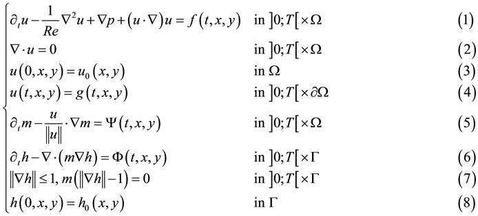
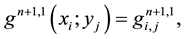
where
・  is the vector velocity, w is the component following the x-axis and v the y-axis one;
・  is the pressure;
・  ,
,  and
and  are the source term;
・  is the mass density;
・  is the height of sand dune;
・  is the Reynolds number;
・ T is a given positive time-parameter.
The out-flow of the fluid is modelling by Equations (1)-(4). The transportation of the sand grains under the effect of averaged velocity is modelling by Equation (5). The dynamics of the sand dune is modelling by Equ- ations (6)-(8).
To ensure the regularity of the solution we suppose that the functions f,  and
and  are square integrable on
  while functions
  and
and  are square integrable on
 . We also suppose that the boundary conditions given by Equation (4) verify the said condition of debit:

and the initial data  must verify:

where n is the unit vector normal to the boundary of the domain .
.
3. Numerical Schemes
3.1. Temporal Discretisation
For a given positif integer r, we consider a time step discretisation , with
 . Then, we define the
knots of the interval  given by
 , with
 .
.
For a given continues function , we approximate
  at the knots
  by:
by: .
.
In order to approach in time Equations (1)-(8), we used second-order backward Euler scheme which is given by:
 (9)
(9)
While doing an extrapolation of order 1 of the pressure at the time of the prediction stage and while appro- aching the convection term  by a numerical scheme of Adams-Bashforth type, the basic principle of the projection methods in [8] [9] applied to Equations (1)-(4), allows us to get:
- prediction stage:
 (10)
(10)
 (11)
(11)
where  denotes the predicted velocity,
  and
and
 ,
,
- projection stage:
 (12)
(12)
 (13)
(13)
 (14)
(14)
where  for
for . This last stage corresponds to a Darcy problem [10] that is as well as the stokes problem of type saddle point.
Thus, when one does a spatial discretisation of this problem by using a Chebyshev spectral method, so that the resulting discreet problem is well posed, it is necessary that the discreet spaces of velocity and pressure verify a compatibility condition inf-sup of Brezzi [11] .
To answer this question of compatibility condition, we use the spectral method  by using only one grid define by the usual Chebyshev-Gauss-Lobatto [12] [13] .
3.2. Spatial Discretisation
In this section we present the basic principle of the method .
.
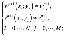
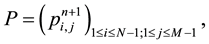
So for a given positive integers N and M we denote by  and
and  sets of orthogonal poly- nomials of degree less than or equal to N and
 , respectively, where
  is an open subset such that
 . Let denote by
 , the set of polynomials defined on
  of degree N according to the variable x and degree M according to the variable y, and
 , the set of polynomials defined on
  of degree
  according to the variable x and degree
  accord- ing to the variable y.
The  method consists in approaching the pressure by orthogonal polynomials of degree less than two units as those approaching the velocity while considering only one grid.
In this paper, we consider Chebyshev polynomials and choose the Chebyshev-Gauss-Lobatto mesh defined by:
 and
and , for
, for  and
and .
.
Then, we consider the velocity at  points of
  and the pressure at
  points insides of
 . Therefore, compatibility between the spaces of approximation of the velocity and the pressure is assured and the condition inf-sup is satisfied [14] [15] .
Let us making the following space approximation for 

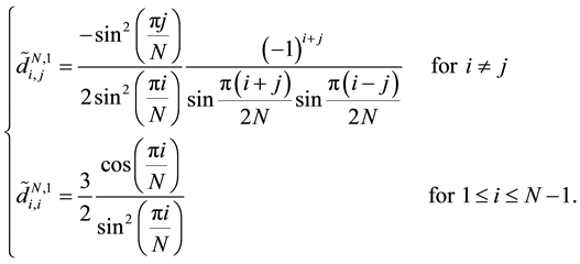
We approach the first and secondary operators of derivation of  in
in  [6] [13] [16] by:


where  and
and  are coefficients of the Chebyshev differentiation matrixes of
order 1  and order 2
 , respectively in
 . We approach the first operators of derivation of pre- ssure p in
  [17] by:


where  are coefficients of the Chebyshev differentiation matrix of order 1
  in
in
 , given by the following relation:
Let us consider the following approximation spaces:


where  and
and  are the first and second component of g, respectively.
We define by:
Then the prediction stage (9)-(10) decomposes itself in two-Helmholtz problems for each components of the predicted velocity with Dirichlet boundary conditions:
 (15)
(15)
 (16)
(16)
 (17)
(17)
 (18)
(18)
The Chebyshev collocation approximation of Helmholtz problems (15) and (17) is given by:
 (19)
(19)
and
 (20)
(20)
Multiplying these equations by , we obtain the following relations given by:
 (21)
(21)
and
 (22)
(22)
where
 ,;
,;
 ;
;
Let us denote by:


Then, we can rewrite Equations (21) and (22) by:
 (23)
(23)
and
 (24)
(24)
 is a matrix
  obtained by suppressing the first and last lines, the first and last columns of the matrix
 .
.
Systems (23) and (24) are solving by using diagonalisation method [10] .
Let us denote by  and
and  the diagonal matrixes whose entries are the eigenvalues
 ,
,  , and
, and ,
,  , of the matrixes
  and
and , respectively, so that
 (25)
(25)
and
 (26)
(26)
where  and
and  are matrixes defined by the eigenvectors.
Multiplying the Equation (23) on the left by , we obtain:
 (27)
(27)
we deduce that:
 (28)
(28)
Let us denote by , the Equation (28) can be rewrite as:
 (29)
(29)
From (25) and (26), we deduce:
 (30)
(30)
and multiplying this equation on the right by , we obtain:
 (31)
(31)
so that, we deduce the following equation:
 (32)
(32)
Denoting by  and
and , Equation (24) becames:
 (33)
(33)
using relation (26), we obtain:
 (34)
(34)
Then, we deduce:
 (35)
(35)
We compute completely  and
and , by using the following algorithm:
1) Compute .
.
2) Compute 
3) Compute  from (27).
4) Compute 
5) Compute 
When applying the same algorithm to Equation (24), we can compute completely .
.
In order to make the projection stage, we define:

then we can rewrite Equations (12)-(13) by:
 (36)
(36)
 (37)
(37)
 (38)
(38)
with boundary conditions:


So, while noting:
then by using spectral method , we obtain the spatial discretisation of Equations (36)-(38) as following :
 (39)
(39)
 (40)
(40)
 (41)
(41)
where ,
, 
with boundary conditions :


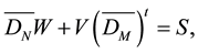
Let us denote by:


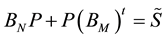
Then, we obtain the following matrix formulation for Equations (39)-(41), given by:
 (42)
(42)
 (43)
(43)
 (44)
(44)
where  is a matrix obtaining by suppressing the first and last lines, the first and last columns of the Cheby- shev matrix of derivation
 .
.
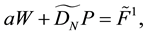
Reformulating Equations (42), (43) and (44), we deduce :
 (45)
(45)
 (46)
(46)
 (47)
(47)
where

We solve Equation (47) by using the same strategy using for solving Equation (21) and (22). Then we deter- mine completely the P matrix for the pressure and deduce the matrixes W and V containing the values of the first and the second components of velocity, respectively from Equations (45) and (46).
Let us denote by  the approximation of the masse density at the mesh
  for
for
 ,
,  and
and . While approaching the first derivation of the density m in
 , and using relation (9), Equation (5) give:
 (48)
(48)
We denote by  the vector given by:

We can rewrite Equation (48) by:
 (49)
(49)
where:


where  is the identity matrix of order
  and
and  the matrix of order
  of entries equal to 1 and
  denotes the velocity of the out-flow.
And while denoting by , we obtain:
 (50)
(50)
To make the approximation of Equations (6)-(8), we suppose that the strong domain occupied by sand dune is
parameterized by , with
  so that this domain is contained in
 .
.
What brings us to consider another grid to approach the dune height by using new grid , defined by:
 and
and , for
, for  and
and .
.
Let us denote by  the approximation of the dune height at the mesh
  for
for
 ,
,  and
and . While approaching the first derivation of the dune height h in
 , and using relation (9), Equation (6) give:
 (51)
(51)
 (52)
(52)
Denoting by  the vector given by:

we obtain the following matrix formulation:
 (53)
(53)
where:


and while denoting by :
 we can rewrite Equation (53):
 (54)
(54)
4. Numerical Result
For the numerical simulation, we consider an experimental solution on the one hand for the Navier-Stokes equations and other for the mass density and the dune height.
For example:


We take ,
,  and
and  for the cases tests. While noting
the calculated fields, we give the evolution of the temporal error  during the time. The
integration in time of this error is initialized while taking the fields to the instants  equals to the exact solution to the same time level.
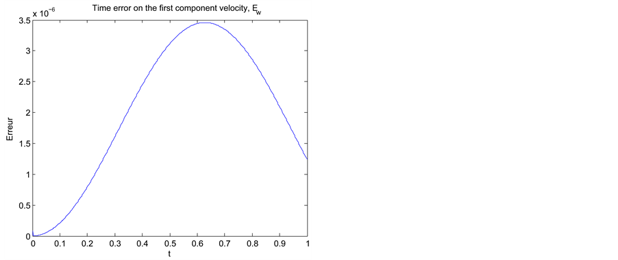
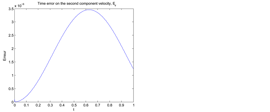
We represent temporal errors according to the first components  (Figure 1(a)) and the second
 (a) (b)
Figure 1. Temporal evolution of the errors in time on the first component of the velocity,  (a), and the second component
  (b), for a step of time
components  (Figure 1(b)) of the velocity by using the following parameters of discretisation
  and
and . One notices a likeness between the two figures, that shows the precision of the second order in time by the numerical scheme used. Also, these errors don’t depend on the chosen of spatial discretisation.
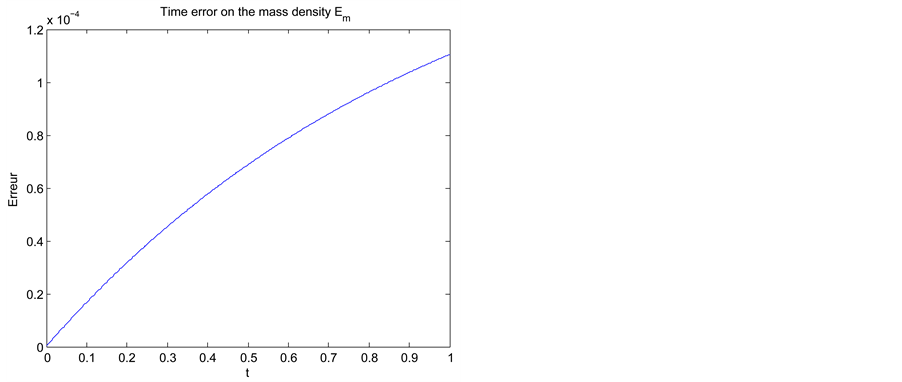
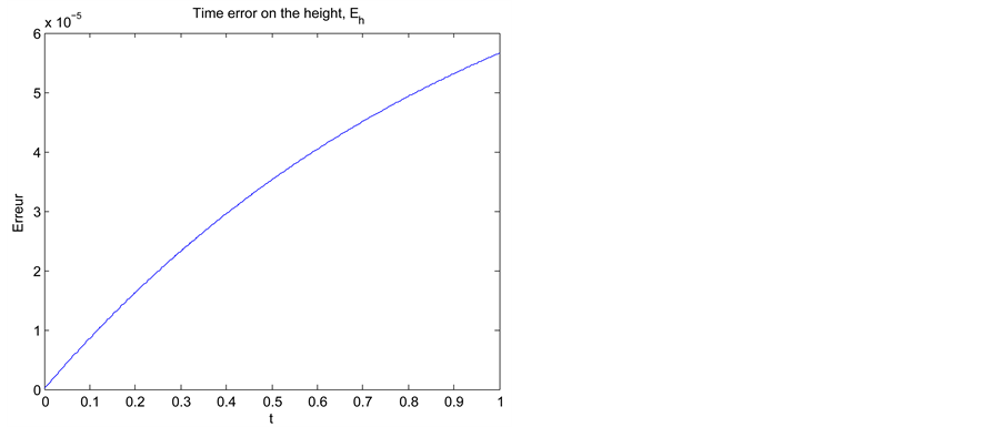
We also represent the temporal errors for the mass density of sand grains  (Figure 2(a)) and the dune height
  (Figure 2(b)) by using
 ,
,  and
and . These also confirm the precision of the second order in time by the numerical scheme used.
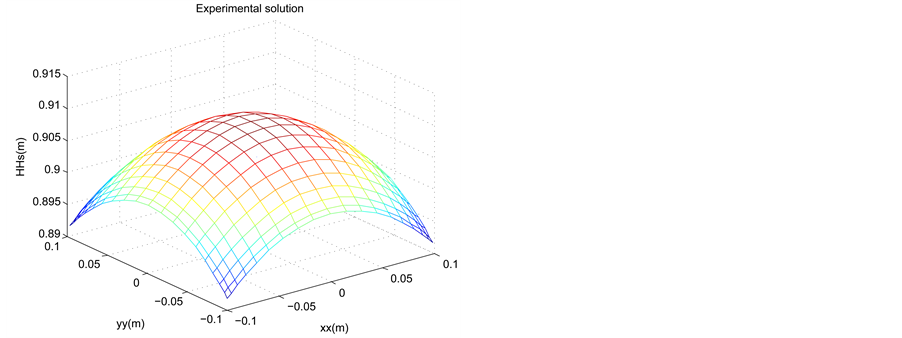
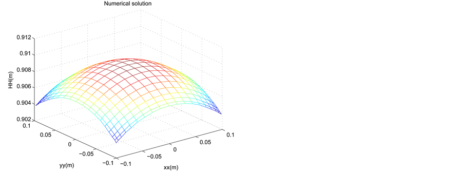
The profile of the dune height is represented at , for
, for  by using
  (Figure 3),
  (Figure 4), and
  (Figure 5). The experimental height on the left and the approach height on the right. One notices that the simulations made for
  give a better approximation of the dune height that those achieved for μ = 10 and
 . That permits us to conclude that for a higher value of parameter μ we obtain a good approximation for a dune height in the strong domain
 . Also, these figures show a likeness between the numerical solution and the experimental solution for each value of parameter
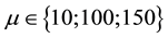 . That permits us to conclude the consistency of our approach.
 (a) (b)
Figure 2. Temporal evolution of the errors in time on the mass density of sand grains,  (a), and on the dune height,
  (b), for a step of time
  and
and
 (a) (b)
Figure 3. Profile of the experimental and approached of the dune height in the space at t = 0.095, for a time step Δt = 5 × 10⁻³, N = M = 20 and
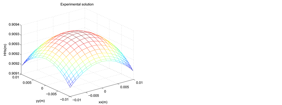
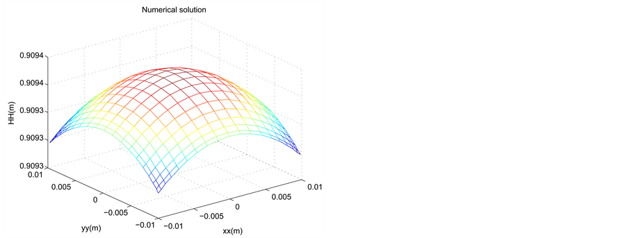
Figure 4. Profile of the experimental and approached of the dune height in the space at t = 0.095, for a time stepΔt = 5 × 10⁻³, N = M = 20 and
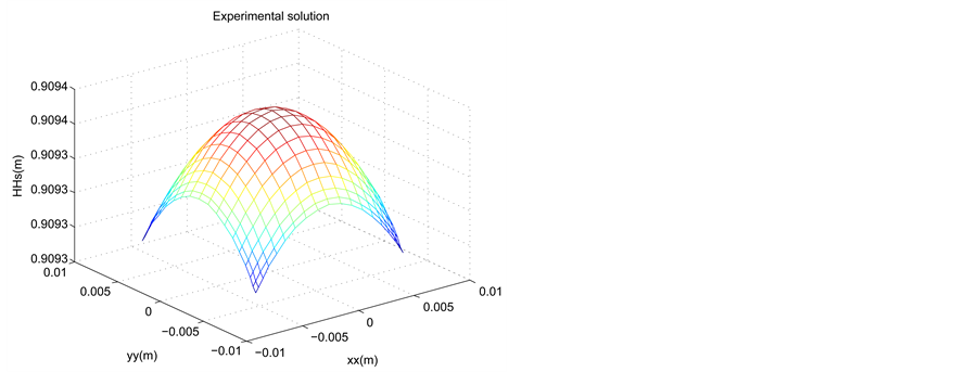
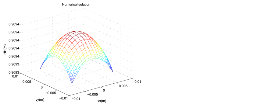
Figure 5. Profile of the experimental and approached of the dune height in the space at t = 0.095, for a time step Δt = 5 × 10⁻³, N = M = 20 and
5. Conclusions and Perspectives
We have solved numerically a mathematical model of sand dune formation in a surface water to incompressible out-flows in two space dimensions. This model couples the Navier-Stokes equations governing the incompressi- ble out-flows in two-dimension of space and the Prigozhin equation that describes the evolution of a sand dune in a surface water. One of the difficulties of this approach resides in the treatment of the pressure which appears only in Navier-Stokes equations as Lagrange multiplier. We used a Chebyshev projection scheme following a spectral approach  to solve the Navier-Stokes equations, which permitted us to ignore the boundary conditions on the pressure. And, as we don’t have any boundary condition on the mass density and the dune height, we have expressed the first and secondary operator derivations in
  for the mass density and in
  for the dune height. It is evident from the gotten results that the smaller the strong domain
  occupied by the dune is, the better the approximation of the dune height is.
In our future works, we count to pass in dimension 3 of space and to put a optimal control in place to deter- mine the optimal height of sand dune in a surface water, from which other dunes can be formed in the fluid.
References
- Prigozhin, L. (1994) Sandpiles and River Networks: Extended Systems with Nonlocal Interactions. Physical Review E, 49, 1161. http://dx.doi.org/10.1103/physreve.49.1161
- Igbida, N. (2012) Mathematical Models for Sandpile Problems. XLIM-DMI, UMR-CNRS 6172, Workshop MathEnv, Essaouira.
- Nouri, Y.M. and Bisso, S. (2013) Numerical Approach for Solving a Mathematical Model of Sand Dune Formation. Pioneer Journal of Advances in Applied Mathematics, 9, 1-15.
- Rønquist, E.M. (1990) Optimal Spectral Element Methods for the Unsteady 3-Dimensionnal Incompressible Navier-Stokes Equations. Ph.D. Thesis, Mass, Cambridge.
- Azaez, M. (1990) Computation of the Pressure in the Stokes Problem for Incompressible Viscous Fluids by a Spectral Method Collocation. Thesis of Doctorate, Paris-Sud University, Orsay.
- Botella, O. (1996) Resolution des equations de Navier-Stokes par des schemas de Projection Tchebychev. Rapport de recherche No. 3018 de L’Institut national de rechercheen informatique et en automatique (inria).
- Maday, Y., Patera, A.T. and Rønquist, E.M. (1992) The
![]() Method for the Approximation of the Stokes Problem. Laboratoire d’Analyse Numerique, Paris VI, 11, fasc.4.>http://html.scirp.org/file/12-7402713x290.png" class="200" /> Method for the Approximation of the Stokes Problem. Laboratoire d’Analyse Numerique, Paris VI, 11, fasc.4.
Method for the Approximation of the Stokes Problem. Laboratoire d’Analyse Numerique, Paris VI, 11, fasc.4.>http://html.scirp.org/file/12-7402713x290.png" class="200" /> Method for the Approximation of the Stokes Problem. Laboratoire d’Analyse Numerique, Paris VI, 11, fasc.4. - Chorin, A. (1968) Numerical Simulation of the Navier-Stokes Equations. Mathematics of Computation, 22, 745-762. http://dx.doi.org/10.1090/S0025-5718-1968-0242392-2
- Temam, R. (1969) On the Approximation of the Solution of Navier-Stokes Equations by the Fractional Steps Method II. Archive for Rational Mechanics and Analysis, 32, 377-385.
- Azaez, M., Bernardi, C. and Grundmann, M. (1994) Spectral Methods Applied to Porous Media Equations. East-West Journal of Numerical Mathematics, 2, 91-105.
- Brezzi, F. (1974) On the Existence, Uniqueness and Approximation of Saddle-Point Problems Arising from Lagrangian Multipliers. R.A.I.R.O, R2, 129-151.
- Hesthaven, J.S., Gottlieb, S. and Gottlieb, D. (2007) Spectral Methods for Time-Dependent Problems. Cambridge University Press, Cambridge. http://dx.doi.org/10.1017/CBO9780511618352
- Trefethen, L.N. (2000) Spectral Methods in MATLAB. http://dx.doi.org/10.1137/1.9780898719598
- Canuto, C., Bernardi, C. and Maday, Y. (1986) Generalized Inf-Sup Condition for Chebyshev Approximation of the Navier-Stokes Equations. Technical Report, No. 86-61, ICASE.
- Canuto, C., Hussaini, M.Y., Quarteroni, A. and Zang, T.A. (1988) Spectral Methods in Fluid Dynamics. Springer- Verlag, New York. http://dx.doi.org/10.1007/978-3-642-84108-8
- Ehrenstein, U. and Peyret, R. (1989) A Chebyshev-Collocation Method for the Navier-Stokes Equations with Application to Double-Diffusive Convection. International Journal for Numerical Methods in Fluids, 9, 427-452. http://dx.doi.org/10.1002/fld.1650090405
- Azaez, M., Fikri, A. and Labrosse, G. (1994) A Unique Grid Spectral Solver of the nd Cartesian Unsteady Stokes System. Illustrative Numerical Results. Finite Elements in Analysis and Design, 16, 247-260. http://dx.doi.org/10.1016/0168-874X(94)90068-X
 Method for the Approximation of the Stokes Problem. Laboratoire d’Analyse Numerique, Paris VI, 11, fasc.4.>http://html.scirp.org/file/12-7402713x290.png" class="200" /> Method for the Approximation of the Stokes Problem. Laboratoire d’Analyse Numerique, Paris VI, 11, fasc.4.