Applied Mathematics
Vol.5 No.16(2014), Article ID:49468,11 pages
DOI:10.4236/am.2014.516244
Asymptotic Harmonic Behavior in the Prime Number Distribution
Maurice H.P.M. van Putten
Sejong University, Seoul, South Korea
Email:mvp@sejong.ac.kr
Copyright © 2014 by author and Scientific Research Publishing Inc.
This work is licensed under the Creative Commons Attribution International License (CC BY).
http://creativecommons.org/licenses/by/4.0/


Received 16 June 2014; revised 19 July 2014; accepted 29 July 2014
Abstract
We consider
 on
on , where the sum
is over all primes
, where the sum
is over all primes . If
. If
 is bounded on
 , then the Riemann
hypothesis is true or there are infinitely many zeros
, then the Riemann
hypothesis is true or there are infinitely many zeros . The first 21 zeros
give rise to asymptotic harmonic behavior in
. The first 21 zeros
give rise to asymptotic harmonic behavior in
 defined by the prime numbers up to one trillion.
Keywords: Prime Number Distribution,Summation,Regularization

1. Introduction
The Riemann-zeta function is the analytic extension of
 (1)
(1)
where Euler’s identity on the right hand side expresses the relation of the integers
to the primes. The zeros
 of Riemann’s analytic continuation of (1) comprise the negative even integers,
 , and an infinite number of nontrivial zeros
 in the strip
 .
.
A general approach to find zeros is by continuation[1]
. If
 is a starting point of a path
 with tangent
 ,
,
 (2)
(2)
then the endpoint
 is a zero of
 , all of which are isolated.
All known nontrivial zeros satisfy
, all of which are isolated.
All known nontrivial zeros satisfy to within numerical precision, the first three of which are
 ,
,

 By the symmetry
 (3)
(3)
it suffices to study zeros in the half plane .
Figure 1illustrates root finding by (2) for the first few zeros.
.
Figure 1illustrates root finding by (2) for the first few zeros.
Continuation (2) is determined by the prime numbers, since
 (4)
(4)
whereby
 (5)
(5)
The poles of
 at the zeros are therefore expressed by the prime number distribution.
In this paper, we study the distribution of zeros
 by Fourier analysis of the function
 (6)
(6)
on , where
 (7)
(7)
with summation over all primes. In what follows, we put
 (8)
(8)
The
 are absolutely summable by Stirling’s formula and
the asymptotic distribution of
are absolutely summable by Stirling’s formula and
the asymptotic distribution of .
.
Theorem 1.1. In the limit as
 becomes small, we have the asymptotic behavior
 (9)
(9)
In (9), is evidently unbounded in the limit as
 approaches zero whenever a finite number of zeros

exists off the critical line .
.
Corollary 1.2. If
 is bounded, then the Riemann hypothesis is true or there are infinitely many zeros
 .
.
A similar relation between the distribution of
 and the primes is [2]
[3]
and the primes is [2]
[3]
 (10)
(10)
based on the Chebyshev functions
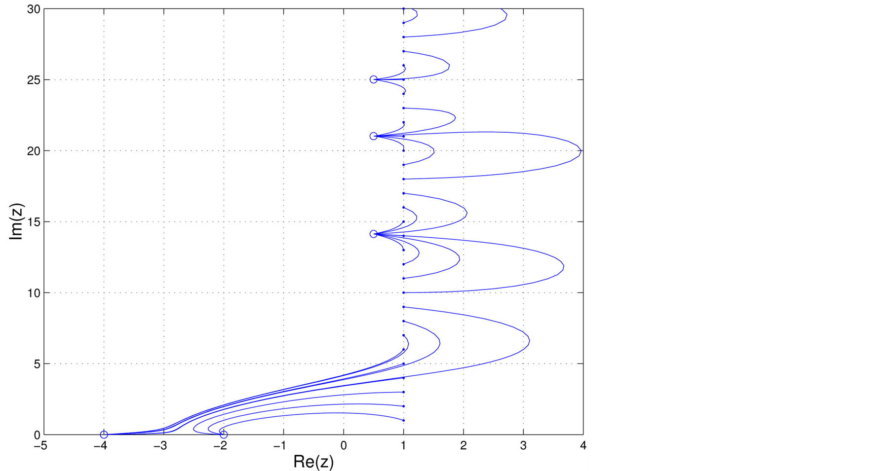
Figure 1.Shown are the
trajectories of continuation
 in the complex plane
 by numerical integration of (2) with initial data

 indicated by small dots on
 . Continuation produces
roots indicated by open circles, defined by finite endpoints of
. Continuation produces
roots indicated by open circles, defined by finite endpoints of
 in the limit as
 approaches infinity. The roots produced by the choice of initial data are the first
three on
approaches infinity. The roots produced by the choice of initial data are the first
three on
 and −2 and −4 of the trivial roots.
 (11)
(11)
where the sum is over all primes
 and integers
 . In (9),
 has a normalization by
 according to and
 is absolutely convergent for all
 , whereas in (10)
 is normalized by
 and the sum
 is not absolutely convergent. Similar to Corollary
1.2, the left hand side of (10) will be bounded in the limit of large
is not absolutely convergent. Similar to Corollary
1.2, the left hand side of (10) will be bounded in the limit of large
 if the Riemann hypothesis is true.
Section 2 presents some preliminaries on . Section 3 gives an integral
representation of
. Section 3 gives an integral
representation of
 and a discussion on its singularity at
 . In Section 4, Cauchy’s
integral formula is applied to derive a sum of residues associated with the
. In Section 4, Cauchy’s
integral formula is applied to derive a sum of residues associated with the . The proof Theorem 1.1
follows from a Fourier transform and asymptotic analysis (Section 5). In Section
6, we illustrate a direct evaluation of
. The proof Theorem 1.1
follows from a Fourier transform and asymptotic analysis (Section 5). In Section
6, we illustrate a direct evaluation of
 using the primes up to one trillion, showing harmonic behavior arising from
 by the first few zeros
 . We summarize our findings
in Section 7.
. We summarize our findings
in Section 7.
2.Background
Our analysis begins with some known properties of
 in, e.g.,[4] -[9]
.
in, e.g.,[4] -[9]
.
Riemann obtained an analytic extension of
 by expressing
 in terms of
 ,
,
 (12)
(12)
where
 (13)
(13)
Here, satisfies
 as
as
 approaches zero by the identity
 for the Jacobi function
 1. On
1. On , it obtains
the meromorphic expression (e.g. Borwein et al., 2006)
, it obtains
the meromorphic expression (e.g. Borwein et al., 2006)
 (14)
(14)
which gives a maximal analytic continuation of
 and shows a simple pole at
 with residue 1.
Riemann further introduced the symmetric form ,
, satisfying
 , whereby
 (15)
(15)
using
 and
and . Along
 ,
, is nonvanishing [10] -[13]
, allowing
is nonvanishing [10] -[13]
, allowing
 (16)
(16)
in terms of the digamma function
 (17)
(17)
in the limit of large .
.
Lemma 2.1. In the limit of large , the logarithmic
derivative of
, the logarithmic
derivative of
 satisfies
 (18)
(18)
Proof. The result follows from (17) and (16). Lemma 2.2.Along the line , we have the asymptotic expansion
 in the limit of large
 , whereby the
 are absolutely summable.
Proof.Recall (8) and the asymptotic expansion
 with a branch cut along the negative real axis. In the limit of large
 ,
, , and hence
 , since
 as
as

becomes large. Hence,the
 are absolutely summable. Numerically, their sum is small,
based on a large number of known zeros .Lemma 2.3. In the
limit of large
.Lemma 2.3. In the
limit of large , we have
 (19)
(19)
Proof. By Lemma 2.1-2.2, we have
 (20)
(20)
 . Also
 (21)
(21)
on
 for some positive constants
 .,
.,
3.An IntegralRepresentation of

Following the same steps leading to the Riemann integral for , we have
 (22)
(22)
where
 absorbs the simple pole in
 at
at
 due to the simple pole in
 at
at , leaving
 analytic at
 . Following a decomposition
 ,
,
 (23)
(23)
and substitution ,
, appears as the Laplace transforms
 (24)
(24)
These integral expressions allow continuations to , respectively, the entire
complex plane.
, respectively, the entire
complex plane.
Lemma 3.1. Analytic extension of
 extends to
 .
.
Proof. With , the second term on the right hand
side in (5) satisfies
, the second term on the right hand
side in (5) satisfies
 (25)
(25)
which is bounded in . Since the second term
 in (5) is analytic in
 , it follows that
 in is analytic on
 . Following (5) as
 approaches
 from the right, we have
 (26)
(26)
where
 is analytic at
 . By (22), as
 approaches
 from the right, we have
 (27)
(27)
where
 is analytic about
 .
Figure 2 shows a numerical evaluation of
.
Figure 2 shows a numerical evaluation of
 for small
 evaluated for the 37.6 billion primes up to one trillion, allowing
 down to

 in view of the requirement for an accurate truncation in
 as defined by (7). The result shows asymptotic harmonic behavior in the limit as
 becomes small.
If the integral
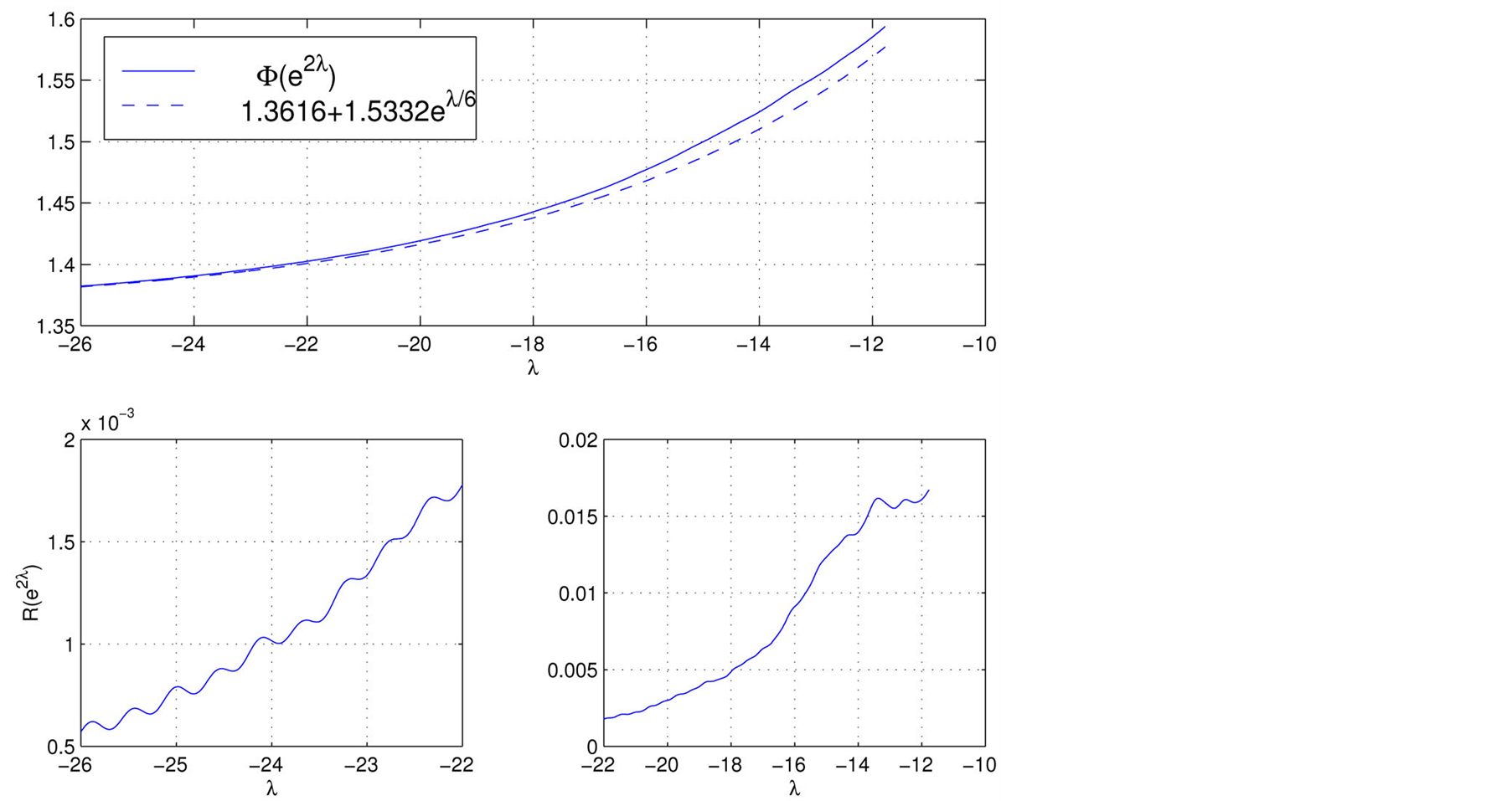
Figure 2.The top window shows
 on
on
 and its leading order approximation
 . The asymptotic harmonic
behavior is apparent in the residual difference (52) between the two, shown in the
bottom two windows, including the period of 2.2496 in
. The asymptotic harmonic
behavior is apparent in the residual difference (52) between the two, shown in the
bottom two windows, including the period of 2.2496 in associated with the first zero
 .
.
 (28)
(28)
is absolutely convergent as
 approaches zero, e.g., when
 is of one sign in some neighborhood of
 , as in the numerical evaluation shown in Figure 2, then
 has an analytic extension into

with no singularities, implying the absence of
 in this region. However, this requires information on the point wise behavior of
 , which goes beyond the relatively weaker integrability
property (23).
, which goes beyond the relatively weaker integrability
property (23).
To make a step in this direction, we next apply a linear transform to (5) to derive
the asymptotic behavior of
 in terms of the distribution
 .
.
4.A Sum of Residues ZAssociated with the Non-Trivial Zeros
Consider
 (29)
(29)
and its Fourier transform
 (30)
(30)
Lemma 4.1. has a simple pole at
 with residue 1 and simple poles at each of the nontrivial zeros
 of
of
 with residue
 .
.
Proof. We have (e.g. Borwein et al. 2006)
 (31)
(31)
where
 is a constant, so that
 (32)
(32)
Here
 (33)
(33)
where
 denotes the digamma function as before, includes contributions from the logarithmic
derivative of the factor to
denotes the digamma function as before, includes contributions from the logarithmic
derivative of the factor to
 in (31), whose singularities are restricted to the trivial zeros of
 . We now consider
the Fourier integral over
. We now consider
the Fourier integral over
 as part of contour integration closed over
 and
and .
.
Proposition 4.2. The Fourier transform of
 over
over
 satisfies
 (34)
(34)
in the limit of large .
.
Proof. Integration over

 gives
gives
 (35)
(35)
where we choose
 to be between two consecutive values of
 . We have
 (36)
(36)
In the limit as
 approaches infinity,
 approaches zero and
 becomes small by Lemma 2.2., whence
 (37)
(37)
Next, integration over
 with a small semicircle around
 obtains an
 result in the limit of large
 by application of Lemma 2.1-2.3 and the Riemann-Lebesgue Lemma. The result now follows
in the limit as
by application of Lemma 2.1-2.3 and the Riemann-Lebesgue Lemma. The result now follows
in the limit as
 approaches infinity, taking into account the residue sum
 associated with the
 and absolute summability of the
 . ,
. ,
5.Proof of Theorem 1.1
Multiplying (5) by , we have
 (38)
(38)
that is, by (22) and (29),
 (39)
(39)
We thus consider
 (40)
(40)
which ab initio is defined on
 by Euler’s identity with Fourier transform
 (41)
(41)
Turning to the right hand side of (40), we consider the coefficients
 (42)
(42)
Here, since
since . In particular,
 and
and
 has a well defined limit and
 in the limit as
 becomes arbitrarily large.
Lemma 5.1. The sum
 is well-defined on
 .
.
Proof. The result follows from the case . By the Prime Number
Theorem,
. By the Prime Number
Theorem, , whereby summation over the tails
 satisfy
 (43)
(43)
whenever . Hence, for
 ,
, whenever
 . It follows that
 (44)
(44)
on .Lemma 5.2.For any
 , the Fourier
transform of
, the Fourier
transform of
 over
over
 satisfies
 (45)
(45)
Proof. The Fourier integral can be obtained in a contour integration with closure
over
 and the edges

 for large
 . In the
notation (42), it obtains a residue
. In the
notation (42), it obtains a residue

at , since
 , whence
 (46)
(46)
The integral (46) exists by virtue of a removable singularity of
 at
at . It asymptotically decays to zero for large
 when
when
 by the Riemann-Lebesgue Lemma. We now consider (40) with (22),
 (47)
(47)
with a remainder
 (48)
(48)
Lemma 5.3. For , the Fourier transform
 (49)
(49)
in the limit of large .
.
Proof. Since
 is analytic in
 , we are at liberty
to consider the transform
, we are at liberty
to consider the transform
 on
on
 . The result follows from the Riemann-Lebesgue
Lemma. Proof of Theorem 1.1. The Fourier transform of (47) is
. The result follows from the Riemann-Lebesgue
Lemma. Proof of Theorem 1.1. The Fourier transform of (47) is
 (50)
(50)
By Proposition 4.2 and Lemmas 5.1-5.2, we have
 (51)
(51)
With , Theorem 1.1 now follows. ,
6.Numerical Illustration of Asymptotic Harmonic Behavior
The harmonic behavior emerges in
 (52)
(52)
To search for higher harmonics
 associated with the zeros
 in
in
 , we compare the spectrum of
 by taking a Fast Fourier Transform with respect to
 ,
,
 (53)
(53)
and compare the results with an analytic expression for the Fourier coefficients
of the
 ,
,
 (54)
(54)
where
 denotes the Bessel function of the first of order
 .
Figure 3 shows the first 21 harmonics in our evaluation of
.
Figure 3 shows the first 21 harmonics in our evaluation of , which is about
the maximum that can be calculated by direct summation in quad precision.
, which is about
the maximum that can be calculated by direct summation in quad precision.
7.Conclusions
The zeros
 of the Riemann-zeta function are endpoints of continuation, defined by an expressed
by a regularized sum
of the Riemann-zeta function are endpoints of continuation, defined by an expressed
by a regularized sum
 over the prime numbers defined by (6).
The zeros
 of
of
 introduce asymptotic harmonic behavior in
 as a function of
 defined by the sum
 of residues of the
 , shown in
Figure 2,Figure 3. Primes up to 4 billion
are needed to identify the first 4 harmonics, up to 70 billion for the 10 and up
to 1 trillion for the first 21. It appears that, effectively, the prime number range
scales exponentially with the number of harmonics it contains.
, shown in
Figure 2,Figure 3. Primes up to 4 billion
are needed to identify the first 4 harmonics, up to 70 billion for the 10 and up
to 1 trillion for the first 21. It appears that, effectively, the prime number range
scales exponentially with the number of harmonics it contains.
Theorem 1.1 describes a correlation between the distribution of the primes and the
distribution of the nontrivial zeros . Suppose there are a finite
number of zeros
. Suppose there are a finite
number of zeros
 in
in . We may then consider
 for which
 gives rise to dominant exponential growth in
 in the limit as
 becomes large. This observation leads to Corollary 1.2.
 can remain bounded in
 only if the Riemann hypothesis is true, or if
 remains fortuitously bounded as an infinite sum over
 with no maximum in
 .
.
Conversely,Riemann hypothesis implies
 (55)
(55)
According to (9) and our numerical calculation shown in
Figure 3,the zeros
 explored to large k by

Figure 3.Shown are the absolute values of the Fourier coefficients
 of
of
 obtained by a Fast Fourier Transform (FFT) of (52) on the computational domain (53),
where
obtained by a Fast Fourier Transform (FFT) of (52) on the computational domain (53),
where ,
, covers 32 periods of
 (dots), on the basis of the 37,607,912,2019 primes up to 1,000,000,000,0039. The
resulting spectrum is compared with the exact spectra
(dots), on the basis of the 37,607,912,2019 primes up to 1,000,000,000,0039. The
resulting spectrum is compared with the exact spectra
 of the
 given by the analytic expression (54) for
 (continuous line). Shown are also the individual spectra of
 for
for
 and 15 associated with the zeros
 ,
, and
and . The match between the computed and exact spectra accurately
identifies the first 21 harmonics of
. The match between the computed and exact spectra accurately
identifies the first 21 harmonics of
 in
in
 out of 22 shown, corresponding to the first 21 nontrivial zeros
 of
of .
.
existing numerical experiments effectively probe (and constrain) a distribution in primes which extends exponentially large in k.
Acknowledgements
The author gratefully acknowledges stimulating discussions with Fabian Ziltener and Anton F.P. van Putten. Some of the manuscript was prepared at the Korea Institute for Advanced Study, Dongdaemun-Gu, Seoul. This research was supported in part by the National Science Foundation through TeraGrid resources provided by Purdue University under grant number TG-DMS100033. We specifically acknowledge the assistance of VickiHalberstadt,RichRaymond and KimberlyDillman. The computations have been carried out using Lahey Fortran 95.
References
- Keller, H.B. (1987) Numerical Methods in Bifurcation Problems. Springer Verlag/Tata Institute for Fundamental Research, Berlin.
- Hadamard, J. (1893) Etude sur les propriétés des fonctions entiéres et en particulier d’une fonction. Journal de Mathématiques Pures et Appliquées, 9, 171-216.
- von Mangoldt, H. (1985) Zu Riemann’s Abhandlung “Über die Anzahl der Priemzahlen unter einer gegebenen Grösse”. Journal für die Reine und Angewandte Mathematik, 114, 255-305.
- Titchmarsh, E.C. (1986) The Theory of the Riemann Zeta-Function. 2nd Edition, Oxford.
- Lehmer, D.H. (1988) The Sum of Like Powers of the Zeros of the Riemann Zeta Function. Mathematics of Computation, 50, 265-273. http://dx.doi.org/10.1090/S0025-5718-1988-0917834-X
- Dusart, P. (1999) Inégalités explicites pour Ψ(X), θ(X), π(X) et les nombres premiers. Comptes Rendus Mathematiques (Mathematical Reports) des l’Academie des Sciences, 21, 53-59.
- Keiper, J.B. (1992) Power Series Expansions of Riemann’s ζ Function. Mathematics of Computation, 58, 765-773.
- Ford, K. (2002) Zero-Free Regions for the Riemann Zeta Function. Number Theory for the Millenium, 2, 25-26.
- Borwein, P., Choi, S., Rooney, B. and Weirathmueller, A. (2006) The Riemann Hypothesis. Springer Verlag, Berlin.
- Littlewood, J.E. (1922) Researches in the Theory of the Riemann ζ-Function. Proceedings of the London Mathematical Society, Series 2, 20, 22-27.
- Littlewood, J.E. (1926) On the Riemann Zeta-Function. Proceedings of the London Mathematical Society, Series 2, 24, 175-201. http://dx.doi.org/10.1112/plms/s2-24.1.175
- Littlewood, J.E. (1928) Mathematical Notes (5): On the Function 1/ζ(1+ti). Proceedings of the London Mathematical Society, Series 2, 27, 349-357. http://dx.doi.org/10.1112/plms/s2-27.1.349
- Wintner, A. (1941) On the Asymptotic Behavior of the Riemann Zeta-Function on the Line . American Journal of Mathematics, 63, 575-580. http://dx.doi.org/10.2307/2371370
- Richert, H.E. (1967) Zur Abschätzung der Riemannschen Zetafunktion in der Nähe der Vertikalen σ = 1. Mathematische Annalen, 169, 97-101. http://dx.doi.org/10.1007/BF01399533
- Cheng, Y. (1999) An Explicit Upper Bound for the Riemann Zeta Function near the Line σ = 1. Rocky Mountain Journal of Mathematics, 29, 115-140. http://dx.doi.org/10.1216/rmjm/1181071682
NOTES

1When
 is an integer,
 is one-half the surface area of
 .
.