Applied Mathematics
Vol.4 No.8(2013), Article ID:35419,10 pages DOI:10.4236/am.2013.48159
Estimation of Regression Model Using a Two Stage Nonparametric Approach
1Department of Statistics, University of Akron, Akron, USA
2Department of Mathematics, College of Charleston, Charleston, USA
Email: *dh52@uakron.edu, *parkj@cofc.edu
Copyright © 2013 Desale Habtzghi, Jin-Hong Park. This is an open access article distributed under the Creative Commons Attribution License, which permits unrestricted use, distribution, and reproduction in any medium, provided the original work is properly cited.
Received April 2, 2013; revised May 2, 2013; accepted May 9, 2013
Keywords: Dimension Reduction; Central Subspace; Polynomial Regression; Shape Restricted
ABSTRACT
Based on the empirical or theoretical qualitative information about the relationship between response variable and covariates, we propose a new approach to model polynomial regression using a shape restricted regression after estimating the direction by sufficient dimension reduction. The purpose of this paper is to illustrate that in the absence of prior information other than the shape constraints, our approach provides a flexible fit to the data and improves regression predictions. We use central subspace to estimate the directions and fit a final model by shape restricted regression, when the shape is known or is stipulated from empirical inspection. Comparisons with an alternative nonparametric regression are included. Simulated and real data analyses are conducted to illustrate the performance of our approach.
1. Introduction
Even if the assumption of monotonicity, convexity or concavity is common, shape restricted regression has not been extensively applied in real applications for two main reasons. As the number of observations , the data dimensionality
 , and the number of constraints
  increases, computational and statistical difficulties (i.e. overfitting) are encountered, refer to [1,2] for detailed discussion. These and other authors proposed different methods to overcome the computational difficulties but there is no optimal solution.
To tackle these limitations, we estimate the direction by the sufficient dimension reduction and fit a final model by the shape restricted regression based on the theoretical shape or stipulated shape of the empirical results. The recent literature for the sufficient dimension reduction proposed practical methods which provide adequate information about the regression with many predictors. Reference [3] considered a general method for estimating the direction in regressions that can be described fully by linear combinations of the predictors without assuming a model for the conditional distribution of , where
 ![]() and
and  are response and explanatory variables, respectively. They also introduced a method to estimate the direction in a single-index regression and [4] extended it to multiple index regression by successive direction extraction.
More specifically, the main goal of this research is to show that the polynomial regression modeling by Central Subspace (CS) and Shape Restriction (SR) methods works well in practice, especially if the scatter plot shows a pattern. As is known that the curve fitting is finding a curve which matches a series of data points and possibly other constraints. This approach is commonly used by scientists and engineers to visualize and plot the curve that best describes the shape and behavior of their data. When more than two dimensions are used, we do not have the luxury of graphical representation any more but have theoretical information about the relationship of the response variable and predictors. Shape restricted regression is a non-parametric approach for building models whose fits are monotone, convex or concave in their covariates. Thses assumptions are commonly applied in biology [5], ranking [6], medicine [7], statistics [8] and psychology [9].
In general, one fits a straight line when the relationship between the response variable and the linear combination of the predictors is linear. Otherwise, one applies polynomial, logarithmic or exponential regression to fit the data. These regressions are practical methodologies when the mean function with predictors is smooth. It is wellknown that the estimation approaches from regression theory are useful in building linear or nonlinear relationships between the values of the predictors and the corresponding conditional mean of the response variable. See [10] for a detailed exposition of widely studied regression methods, particularly polynomial regression. However, the straightforward and efficient analysis may not be generally possible with many predictors. In many situations when the underlying regression function or scatter plot has a particular shape or form, the fitted model can be characterized by certain order or shape restrictions. In this case, the shape restricted classes of regression function are preferred. This nonparametric regression method provides a flexible fit to the data and improves regression predictions.
In addition, when the empirical results between the response and predictors appear to have a particular shape that has certain order or shape restrictions, the shape restricted regression functions may best explain the relationships. Taking shape restrictions into account, one can reduce the model root mean square error or increase the power of the test. This improves the efficiency of a statistical analysis, provided that the hypothesized shape restriction actually holds [11].
In order to contextualize the goal of this article, it is necessary to review the concept of CS and SR. In Section 2, we summarize the notion of CS and an estimation method of CS when the dimension ![]() is assumed to be known. Also, we suggest a data dependent approach to detect the unknown dimensions. In Section 3, we review the shape restricted regression and the constraint cone, over which we minimize the sum of squared errors of our approach for one dimension case. We apply our new approach to the simulated and a real data in Section 4. There are a few comments and concluding remarks in Section 5.
is assumed to be known. Also, we suggest a data dependent approach to detect the unknown dimensions. In Section 3, we review the shape restricted regression and the constraint cone, over which we minimize the sum of squared errors of our approach for one dimension case. We apply our new approach to the simulated and a real data in Section 4. There are a few comments and concluding remarks in Section 5.
2. Estimation Method by Central Subspace
Let ![]() be a scalar response variable and
be a scalar response variable and  be a
be a  covariate vector. Suppose the goal is to make an inference about how the conditional distribution
  varies with the values of
 . Then, the sufficient dimension reduction method is to find the number of linear combinations,
  , for
, for  such that the conditional distribution of
  is the same as the conditional distribution of
 . In other words, there would be no loss of information of predictors if
  were replaced by the
  linear combinations. This is equivalent to finding a
  matrix
  such that
![]() (1)
(1)
where  indicates independence, (1) holds when
  is a matrix whose columns form a basis for the subspace of
 . Therefore, a Dimension Reduction Subspace (DRS) for
 ![]() on
on  is defined as any subspace
  of
of , for which (1) holds. Here
  is defined as the space spanned by the columns of
 . That is, (1) represents that
 ![]() is independent of
is independent of  given
given  and
and  vector
  can be replaced by the
 ![]() vector
vector . This indicates a useful reduction in the dimension of
 , where all the information in
  about
about ![]() is included in the
is included in the  -linear combinations. Here, (1) holds trivially for
  and a dimension reduction subspace always exists. Hence, if the intersection of DRSs is itself a DRS, the Central Subspace (CS) is defined as the intersection of all DRSs, which is written as
  for dimension
 ![]() and
and . That is, CS is the minimum DRS that preserves the original information relating to the data.
In this article, we use a method for estimating the CS,  , which does not require a pre-specified model for
 . If dimension
  of CS are known, we need to estimate only the set of vectors
 . The ultimate goal of this paper is to use these estimated vectors to fit a final model using SR, discussed in Section 3. While [12] considered multivariate kernel estimation of the predictor density, the method introduced in this paper uses one predictor at a time. As a result, it can reduce the computational complexity and avoid the sparsity caused by high-dimensional kernel smoothing.
Suppose a matrix  with
with  and define an information index
  by
by
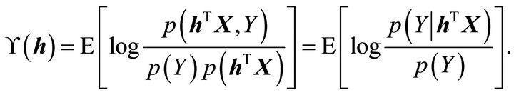 (2)
(2)
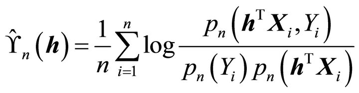
The two forms in (2) are the informational correlation and the expected conditional log-likelihood, respectively. The idea behind this setting is to maximize the information index ![]() over all
over all  matrices
  when
when . Because
  does not involve
 , maximizing
  is equivalent to maximizing the expected conditional log-likelihood. This information index is similar to the Kullback-Leibler information between the joint density
  and the product of the marginal densities
 , quantifying the dependence of
 ![]() on
on . The important properties of the above information index
  is supported by Proposition 1 of [4].
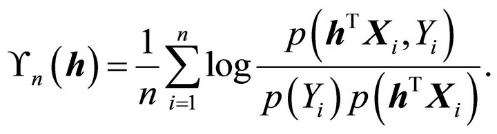
The computation starts to maximize the sample version of ![]() to estimate a basis for the CS. If all the densities were known, a sample version
to estimate a basis for the CS. If all the densities were known, a sample version  of
of  is
is
 is maximized over all
  matrices
 . Because the densities in
  are practically unknown, we use the nonparametric approach to estimate one-dimensional and multi-dimensional density estimates. Here, for the choice of kernels and selection of bandwidths, we follow the general guideline proposed by [13]. Since the Gaussian kernel performed well for the simulated and real data sets, we use density estimates based on a Gaussian kernel for the one-dimensional density and a product of Gaussian kernels for the multi-dimensional densities. Let
  be the univariate Gaussian kernel,
  be the
 ![]() vector, and
vector, and  be the
  observation. Then the
 ![]() -dimensional density estimate has the following form:
-dimensional density estimate has the following form:
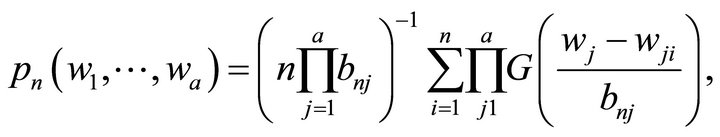 (3)
(3)
where  for
for .
.  is the corresponding sample standard deviation of
  and the constant
 is the optimal bandwidth in the sense of minimizing the mean integrated square error from [13]. The density in
  is replaced by the estimates defined in (3) and maximize (4) for all
  matrices
  such that
 .
.
 (4)
(4)
This method incorporates 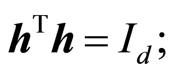 it is the sequential quadratic programming procedure of [14].
Since prior information about ![]() may not be available in practice, it will be useful to find a simpler way to determine
may not be available in practice, it will be useful to find a simpler way to determine ![]() using the data. The sufficient dimension reduction methods have been proposed for the determination of the minimal dimension
using the data. The sufficient dimension reduction methods have been proposed for the determination of the minimal dimension ![]() of the CS. See [15-17] for details. In this paper, using the estimating function
of the CS. See [15-17] for details. In this paper, using the estimating function  defined in (4), we suggest the following Akaike Information Criterion (AIC) to determine
![]() .
.
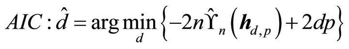 (5)
(5)
3. Fitting Model with Shape Restricted Regression
In this section, we review some fundamental concepts that can help us to lay the groundwork for the construction of the shape restricted method. More details about the properties of the constraint cone and polar cones can be found in [11,18-21].
Suppose we have the following model
where  and
and 
In this model the errors![]() ’s are independent and have standard normal distribution.
’s are independent and have standard normal distribution.  can be monotone, convex or concave based on the qualitative information about the relationship between response variable and predictors or empirical results.
For simplicity let  and
and  For
For  see [20,22] for detailed discussion. The constrained set over which we minimize the sum of squared errors is constructed as follows: the monotone nondecreasing constraints can be written as
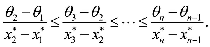
The restriction of  to the set of convex functions is accomplished by the inequalities
In our case,  is a realized value of the linear combination of the predictors;
  is estimated using CS. Any of these sets of inequalities defines
 ![]() half spaces in
half spaces in , and their intersection forms a closed polyhedral convex cone in
 . The cone is designated by
  for
for ![]() constraint matrix
constraint matrix . Here,
  for monotone, nondecreasing convex and
  for convex.
For monotone constraints, the nonzero elements of the ![]() dimensional constraint matrix
dimensional constraint matrix  are
are  and
and  for
for  For convex constraints the nonzero elements of
  are
are 
 and
and  for
for 
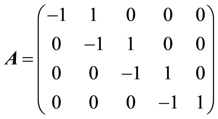
For example, if , the monotone constraint matrix
  is given by
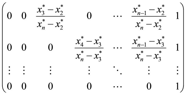
If  and the
 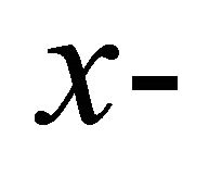 coordinates are equally spaced, the nondecreasing concave and convex constraints are given by the following constraint matrices, respectively:
and
Some computational details: The ordinary leastsquares regression estimator is the projection of the data vector ![]() on to a lower-dimensional linear subspace of
on to a lower-dimensional linear subspace of . In contrast the shape restricted estimator can be obtained through the projection of
 ![]() on to an
on to an ![]() dimensional polyhedral convex cone in
dimensional polyhedral convex cone in  [23]. We have the following useful proposition which shows the existence and uniqueness of the projection of the vector
 ![]() on a closed convex set (see [11]).
on a closed convex set (see [11]).
Proposition 1 Let  be a closed convex subset of
1) For  and
and , the following properties are equivalent:
a) 
b) 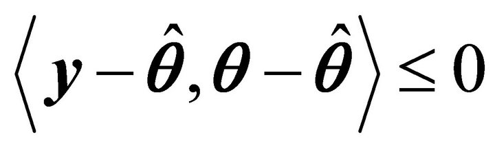 for all
2) For every , there exists a unique point where
  satisfies (a) and (b).
 ![]() is said to be the projection of
is said to be the projection of ![]() onto
onto where the notation
  refers to the vector inner product of
 ![]() and
and . It is easy to see that
 ![]() of Proposition
of Proposition  becomes
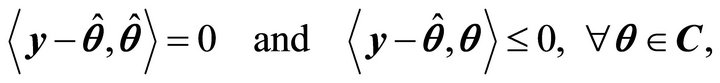 (6)
(6)
which are the necessary and sufficient conditions for ![]() to minimize
to minimize  over
over .
.
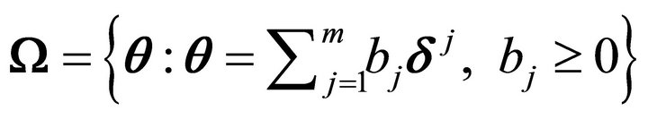
Let  be the linear space spanned by
  for a monotone, nondecreasing convex, and nondecreasing concave, and let
  be the linear space spanned by
  and
and  for convex regression. Note that
  in both cases. The constraint cone can be specified by a set of linearly independent vectors
  as
as
 and the constraint set as
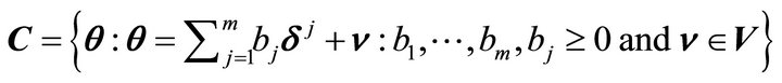 where
where  for monotone, nondecreasing concave, nondecreasing convex and
  for convex. The vectors
  can be obtained from the formula
 . For example, any convex vector
  is a nonnegative linear combination of the
  vectors plus a linear combination of
  and
and .
.
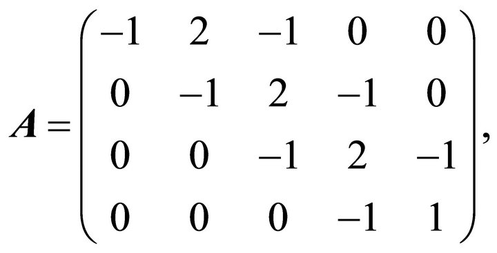
If  is the set of all convex vectors in
 , we can also define the vectors
  to be the rows of the following matrix:
For a large data set, it is better to use the above vectors  because the previous method of obtaining the edges is computationally intensive. Another advantage is that the computations of the inner products with the second approach are faster because of all the zero entries in the vectors.
The polar cone of the constraint cone  is ([19], p. 121)
Geometrically, the polar cone is the set of points in  which make an obtuse angle with all points in
 . Let us note some straightforward properties of
 :
:
1)  is a closed convex cone2) The only possible element in
  is 03)
 .
.
where  is negative rows of
 , i.e.,
  The following proposition is a useful tool for finding the constrained least squares estimator. Its proof was discussed in detail by [23].
Proposition 2 Given  such that
 , the projection of
 ![]() onto the constraint set
onto the constraint set  is
is
 (7)
(7)
and the residual vector  is the projection of
 ![]() onto the polar cone
onto the polar cone .
.
If the set ![]() is determined, using Proposition 2, the constrained least squares estimate,
is determined, using Proposition 2, the constrained least squares estimate, ![]() , can be found through ordinary least-squares regression (OLS), using
, can be found through ordinary least-squares regression (OLS), using  and
and  for
for  as regressors. It is clear that the number of iterations is finite, as there is only a finite number of faces of the cone. To find the set
 ![]() and
and![]() , the mixed primal-dual bases algorithm of [18] or the hinge algorithm of [23] can be used. For monotone regression the pooled adjacent violators algorithm, known as PAVA [11] may be used. A code of the algorithm was written in R. The code can be obtained from the authors upon request.
, the mixed primal-dual bases algorithm of [18] or the hinge algorithm of [23] can be used. For monotone regression the pooled adjacent violators algorithm, known as PAVA [11] may be used. A code of the algorithm was written in R. The code can be obtained from the authors upon request.
4. Numerical Illustration
We examined the performance of the proposed methodology using a real and four simulated data sets. For each of the simulated data set, we carried out the computational algorithms as described in Sections 2 and 3 for sample size n = 100. Recently, [24] investigated a sufficient dimension reduction for different sample sizes and dimensions in the time series context. They found that the performance to detect a true dimension is improved as sample size increases and the computation is more intensive for higher dimensions such as  and 3. For the first three examples, we simulated four data sets which have the worst scenario,
  , and computationally less intensive dimensions,
  and 2 only, to illustrate clearly how the shape restricted method works well in these directions. For the nonparametric alternative we used a kernel. Although optimal bandwidth selection is essential, we used data adaptive fixed bandwidth
 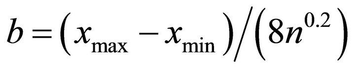 that was recommended by [25]. Here
  and
and  are the maximum and minimum values used in estimation, respectively, and n is the sample size.
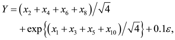
We considered quadratic regression models of a linear combination of six predictors for the first example and ten predictors for the second example. In the third example, we simulated data from cubic regression of a linear combination with ten predictors. The fourth example is more complicated data simulated from two dimensional model including ten predictors. In all the simulated data sets, ![]() are independent standard normal random variables. Finally, we applied our new approach to a real data set, Highway Accident Data.
are independent standard normal random variables. Finally, we applied our new approach to a real data set, Highway Accident Data.
Example 1: Model 1
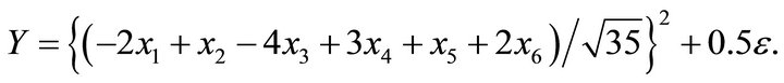
We simulated data from the above model where the mean function is a quadratic function of a linear combination with six predictors. First, we estimated the dimension and direction by CS combined with AIC (5) as described in Section 2. As shown in Table 1, we detected a true dimension . We estimated a vector,
  by the algorithms described in Section 2. The scatter plot,
  vs
vs![]() , shows a quadratic relation, see Figure 1. Then, based on the scatter plot, we fitted the data using convex regression (SR). The decision to use the convex regression was based on a visual examination of the scatter plot.
, shows a quadratic relation, see Figure 1. Then, based on the scatter plot, we fitted the data using convex regression (SR). The decision to use the convex regression was based on a visual examination of the scatter plot.
Example 2: Model 2
In this model, we considered another quadratic mean function of one linear combination with ten predictors. Using the same procedures as the previous example, we estimated dimension and direction by CS. Based on AIC, a true dimension  was detected, see Table 1 for details. The estimated vector is
 .
.
The scatter plot of Figure 2,  vs
vs![]() , shows quadratic relation. The scatter plot suggested that a reasonable choice of the relationship between the
, shows quadratic relation. The scatter plot suggested that a reasonable choice of the relationship between the 
and ![]() is a convex curve. Hence, we fitted a model using convex regression. Figure 2 shows that the shape restricted regression fits the data better than kernel regression, which leads to a smaller error sum of squares.
is a convex curve. Hence, we fitted a model using convex regression. Figure 2 shows that the shape restricted regression fits the data better than kernel regression, which leads to a smaller error sum of squares.
Example 3: Model 3
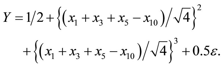
In this example, we simulated data from a cubic polynomial model of one linear combination with ten predictors. In the first step, we estimated dimension and direction by CS. Table 1 indicated that a true dimension  was detected by AIC. The estimated vector is
 .
.
The scatter plot,  vs
vs![]() , shows a cubic curve. In the second step, we fitted a model by concave-convex regression based on the shape of the scatter plot. Our estimator was computed by minimizing the sum of squared errors over the concave-convex set. The inflection point was found by minimizing the sum of squared errors until the conditions in (6) were satisfied. Here, the shape restricted regression does fairly well in all ranges of the data set. The SR and kernel regression are almost on top of each other in the entire range of the data. See Figure 3 and Table 1 for details.
, shows a cubic curve. In the second step, we fitted a model by concave-convex regression based on the shape of the scatter plot. Our estimator was computed by minimizing the sum of squared errors over the concave-convex set. The inflection point was found by minimizing the sum of squared errors until the conditions in (6) were satisfied. Here, the shape restricted regression does fairly well in all ranges of the data set. The SR and kernel regression are almost on top of each other in the entire range of the data. See Figure 3 and Table 1 for details.
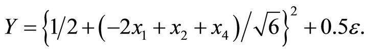
Example 4: Model 4
where  and
and . Here, we consider a nonlinear function including two dimensions. Table 1 showed that we estimated true dimensions
  by AIC. The two directions are

and
 .
.
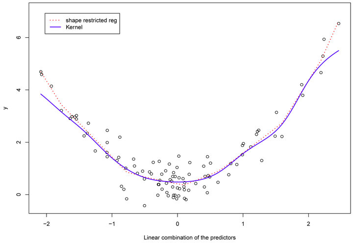
Figure 1. (Model 1) Data are generated from quadratic function of a linear combination with six predictors. The solid curve is quadratic fit and the dotted curve is the shape restricted fit.

Figure 2. (Model 2) Data are generated from quadratic function of a linear combination with ten predictors. The solid curve is quadratic fit and the dotted curve is the shape restricted fit.
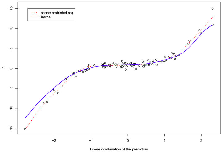
Figure 3. (Model 3) Data are generated from cubic function of a linear combination with six predictors. The solid curve is cubic fit and the dotted curve is the shape restricted fit.
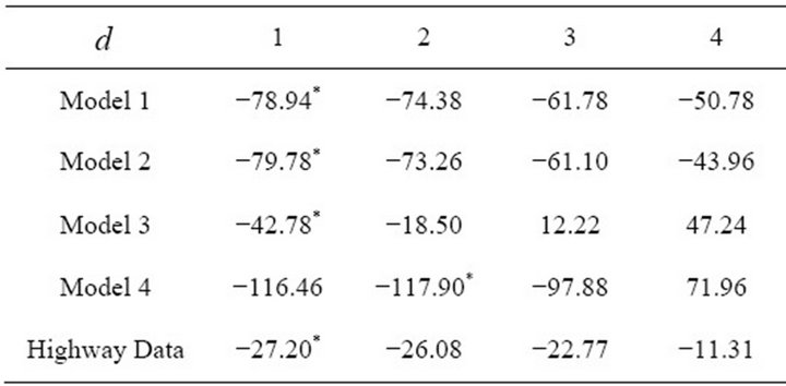
Table 1. AIC values for the simulated and a real data sets using Equations (5).
The response variable Y is non-decreasing in both predictors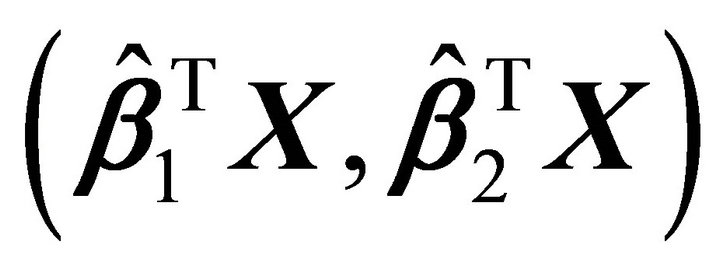 . In addition, the marginal scatter plots,
  vs
vs ![]() and
and 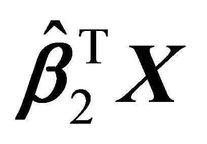 vs
vs![]() , display an increasing trends. Next, we fitted a model by a multiple isotonic regression. The isotonic fit is shown in Figure 4. This shows that our approach may be a better choice than parametric or nonparametric models that do not use the constraints and works well even for two dimensional model.
, display an increasing trends. Next, we fitted a model by a multiple isotonic regression. The isotonic fit is shown in Figure 4. This shows that our approach may be a better choice than parametric or nonparametric models that do not use the constraints and works well even for two dimensional model.
For the purpose of comparison, we computed Average Squared Error Loss (ASEL) of our models and alternative kernel regressions as the following:
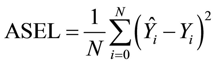
The entries of the Table 2 are the square roots of the ASEL. The results from Table 2 demonstrate that our method performed fairly well in all cases. It is better than kernel regression, in particular, when the data is generated from quadratic and cubic regressions. In general, we can see that our method provides better or comparable fits for the simulated examples, which is also supported by the results of Figures 1-3.
Example 4: Highway Accident Data For illustration, we applied our method to a real data set, Highway Accident Data. See Weisberg (2005) for a detailed description about this data. The data include 39 sections of large highways in the state of Minnesota in 1973 and the variables relate the automobile accident rate in accidents per million vehicle miles to several potential terms. We use log(Rate) as a response variable and eleven terms as explanatory variables. The definition of terms of this data is described in Table 10.5 of Weisberg (2005).
First, we estimated the direction of the predictor variables without losing any information using CS. As shown in Table 2, the dimension  is detected by AIC. The estimated direction is
 .
.
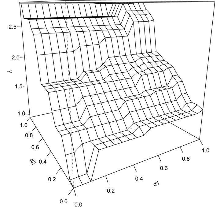
Figure 4. (Model 4) Data are generated from nonlinear mean function which has two dimensional model including ten predictors.
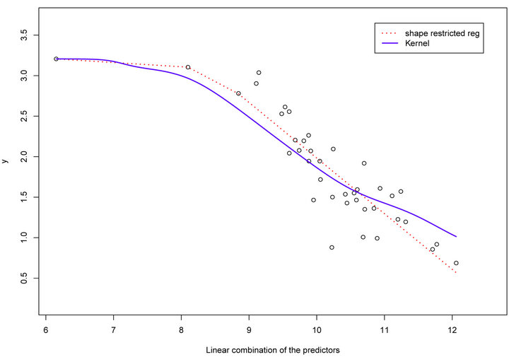
Figure 5. Highway Accident Data: The solid line is cubic fit and and the dotted line is the shape restricted fit.
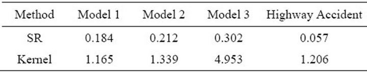
Table 2. Average Squared Error Loss (ASEL) of the shape restricted regression and kernel regression.
From the scatter plot of Figure 4, there is some curvature in the relationship between  vs
vs![]() . Hence, a concave curve may be a good choice to reflect the relationship between the response variable and the linear combination of the predictors. Figure 4 shows the concave and cubic regression fits. The plot of Figure 5 and the ASEL in Table 2 suggests that our method gives reasonable fit to this data set.
. Hence, a concave curve may be a good choice to reflect the relationship between the response variable and the linear combination of the predictors. Figure 4 shows the concave and cubic regression fits. The plot of Figure 5 and the ASEL in Table 2 suggests that our method gives reasonable fit to this data set.
5. Comments
The polynomial regression is one of handy methods in regression analysis. However, this straightforward analysis is not generally possible with many predictors. Hence, the major message that we would like to deliver in this paper is that the estimation of direction by CS and fitting the model by SR is advantageous for high dimensional data that has many predictors. After estimating the direction by sufficient dimension reduction, it is not easy to choose the appropriate polynomial regression model from the pattern of the scatter plot without any theoretical basis. Furthermore, the parametric or nonparametric models that do not use the constraints are not capable of giving different shapes of actual fit such as bimodal function and concave-convex. For such conditions, when the only available information is the shape (decreasing, increasing, concave, convex or bathtub) of the underlying regression function, our approach provides more acceptable fits/estimates.
6. Acknowledgements
Jin-Hong Park is supported in part by the faculty research and development at the Mathematics Department and the College of Charleston.
REFERENCES
- R. Luss, S. Rosset and M. Shahar, “Decomposing Isotonic Regression for Efficiently Solving Large Problems,” Proceedings of the Neural Information Processing Systems Conference, Vancouver, 6-9 December 2010, pp. 1513-1521.
- W. Maxwell and J. Muckstadt, “Establishing Consistent and Realistic Reorder Intervals in Production-Distribution Systems,” Operations Research, Vol. 33, No. 6, 1985, pp. 1316-1341. doi:10.1287/opre.33.6.1316
- X. Yin and R. D. Cook, “Direction Estimation in SingleIndex Regressions,” Biometrika, Vol. 92, No. 2, 2005, pp. 371-384. doi:10.1093/biomet/92.2.371
- X. Yin, B. Li and R. D. Cook, “Successive Direction Extraction for Estimating the Central Subspace in a Multiple-Index Regression,” Journal of Multivariate Analysis, Vol. 99, No. 8, 2008, pp. 1733-1757. doi:10.1016/j.jmva.2008.01.006
- G. Obozinski, G. Lanckriet, C. Grant, M. Jordan and W. Noble, “Consistent Probabilistic Outputs for Protein Function Prediction,” Genome Biology, Vol. 9, No. 1, 2008, pp. 247-254. doi:10.1186/gb-2008-9-s1-s6
- Z. Zheng, H. Zha and G. Sun, “Query-Level Learning to Rank Using Isotonic Regression,” 46th Annual Allerton Conference on Communication, Control, and Computing, Allerton House, 24-26 September 2008, pp. 1108-1115.
- M. J. Schell and B. Singh, “The Reduced Monotonic Regression Method,” Journal of the American Statistical Association, Vol. 92, No. 437, 1997, pp. 128-35. doi:10.1080/01621459.1997.10473609
- R. Barlow and H. Brunk, “The Isotonic Regression Problem and Its Dual,” Journal of the American Statistical Association, Vol. 49, No. 5, 1972, pp. 784-789.
- J. Kruskal, “Multidimensional Scaling by Optimizing Goodness of Fit to a Nonmetric Hypothesis,” Psychometrika, Vol. 29, No. 1, 1964, pp. 1-27. doi:10.1007/BF02289565
- S. Weisberg, “Applied Linear Regression,” Wiley, Hoboken, 2005.
- T. Robertson, F. T. Wright and R. L. Dykstra, “Order Restricted Statistical Inference,” John Wiley & Sons, New York, 1988.
- Y. Xia, “A Constructive Approach to the Estimation of Dimension Reduction Directions,” The Annals of Statistics, Vol. 35, No. 6, 2007, pp. 2654-2690. doi:10.1214/009053607000000352
- D. W. Scott, “Multivariate Density Estimation: Theory, Practice, and Visualization,” John Wiley & Sons, New York, 1992. doi:10.1002/9780470316849
- P. Gill, W. Murray and M. H. Wright, “Practical Optimization,” Academic Press, New York, 1981.
- K. C. Li, “On Principal Hessian Directions for Data Visualization and Dimension Reduction: Another Application of Stein’s Lemma,” Annals of Statistics, Vol. 87, No. 420, 1992, pp. 1025-1039.
- J. R. Schott, “Determining the Dimensionality in Sliced Inverse Regression,” Journal of the American Statistical Association, Vol. 89, No. 425, 1994, pp. 141-148. doi:10.1080/01621459.1994.10476455
- Y. Xia, H. Tong, W. K. Li and L. X. Zhu, “An Adaptive Estimation of Dimension Reduction,” Journal of the Royal Statistical Society, Ser. B, Vol. 64, No. 3, 2002, pp. 363-410. doi:10.1111/1467-9868.03411
- D. A. S. Fraser and H. Massam, “A Mixed Primal-Dual Bases Algorithm for Regression under Inequality Constraints. Application to Convex Regression,” Scandinavian Journal of Statistics, Vol. 16, 1989, pp. 65-74.
- R. T. Rockafellar, “Convex Analysis,” Princeton University Press, 1970.
- E. Seijo and B. Sen, “Nonparametric Least Squares Estimation of a Multivariate Convex Regression Function,” Annals of Statistics, Vol. 39, No. 2, 2011, pp. 1633-1657. doi:10.1214/10-AOS852
- M. J. Silvapulle and P. K. Sen, “Constrained Statistical Inference, Inequality, Order, and Shape Restrictions,” Wiley, New York, 2005.
- M. C. Meyer, “Inference for Multiple Isotonic Regression,” Technical Report, Colorado State Uinversity, 2010.
- M. C. Meyer, “An Extension of the Mixed Primal-Dual Bases Algorithm to the Case of More Constraints than Dimensions,” Journal of Statistical Planning and Inference, Vol. 81, No. 1, 1999, pp. 13-31. doi:10.1016/S0378-3758(99)00025-7
- J.-H. Park, T. Sriram and X. Yin, “Dimension Reduction in Time Series,” Statistica Sinica, Vol. 20, 2010, pp. 747- 770.
- H.-G. Muller and J.-L. Wang, “Hazard Rate Estimation under Random Censoring with Varying Kernels and Bandwidths,” Biometrics, Vol. 50, No. 1, 1994, pp. 61-76. doi:10.2307/2533197
NOTES
*Corresponding author.