Applied Mathematics
Vol.4 No.4(2013), Article ID:30706,8 pages DOI:10.4236/am.2013.44093
Condition for Successful Square Transformation in Time Series Modeling
1Department of Statistics, Faculty of Science, Federal University Otuoke, Yenagoa, Nigeria
2Department of Statistics, Faculty of Biological and Physical Sciences, Abia State University, Uturu, Nigeria
Email: *ohakwej@fuotuoke.edu.ng
Copyright © 2013 J. Ohakwe et al. This is an open access article distributed under the Creative Commons Attribution License, which permits unrestricted use, distribution, and reproduction in any medium, provided the original work is properly cited.
Received January 7, 2013; revised March 4, 2013; accepted March 11, 2013
Keywords: Error Component; Multiplicative Time Series Model; Square Transformation; Moments
ABSTRACT
In this study we establish the probability density function of the square transformed left-truncated  error component of the multiplicative time series model and the functional expressions for its mean and variance. Furthermore the mean and variance of the square transformed left-truncated
  error component and those of the untransformed component were compared for the purpose of establishing the interval for σ where the properties of the two distributions are approximately the same in terms of equality of means and normality. From the results of the study, it was established that the two distributions are normally distributed and have means
  correct to 1 dp in the interval 0 < σ < 0.027, hence a successful square transformation where necessary is achieved for values of σ such that 0 < σ < 0.027.
1. Introduction
Consider a normally distributed random variable X with probability density function  specified as

 (1)
(1)
Often in practice, the random variable X which has a  distribution do not admit values less than or equal to zero. We therefore disregard or truncate all values of
  to take care of the admissible region X > 0. Now if the values of X below or equal to zero cannot be observed due to censoring or truncation, then the resulting distribution is a left-truncated normal distribution.
[1] obtained the probability density function of the left-truncated normal distribution as
 (2)
(2)
with mean  and variance
  given by
 (3)
(3)
and
 (4)
(4)
The study of the properties of normally distributed random variables when certain outcomes are constrained or restricted has been a rich and fertile one—with applications in regression analysis, inventory management and time series modeling to mention but a few.
A time series is a collection of observations made sequentially in time. Examples occur in a variety of fields, ranging from economics to engineering and methods of analyzing time series constitute an important area of statistics [2]. Time series analysis comprises methods that attempt to understand such time series, often either to understand the underlying context of the data points (Where did they come from? What generated them?), or to make forecasts. Time series forecasting is the use of a model to forecast or predict future events based on known past events.
Methods for time series analyses are often divided into three classes: descriptive methods, time domain methods and frequency domain methods. Frequency domain methods centre on spectral analysis and recently wavelet analysis [3,4] can be regarded as model-free analyses. Time domain methods [5,6] have a distribution-free subset consisting of the examination of the autocorrelation and cross-correlation analysis.
Descriptive methods [2,7] involve the separation of an observed time series into components representing trend (long term direction), the seasonal (systematic, calendar related movements), cyclical (long term oscillations or swings about the trend) and irregular (unsystematic, short term fluctuations) components. The descriptive method is known as time series decomposition. If short period of time are involved, the cyclical component is superimposed into the trend [2] and the observed time series  can be decomposed into the trendcycle component
 , seasonal component
  and the irregular/residual component
 .
.
The decomposition model of interest in this study is the multiplicative time series model given by
 (5)
(5)
where  are independent, identically distributed normal errors with mean 1 and variance
  .
.
Data transformation is a mathematical operation that changes the measurement scale of a variable. Reasons for transformation include stabilizing variance, normalizing, reducing the effect of outliers, making a measurement scale more meaningful, and to linearize a relationship [8]. For further details on reasons for transformation, see [9- 11]. Many time series analyst assume normality and it is well known that variance stabilization implies normality of the series. The most popular and common data transformations are the power transformation namely the logarithm, square root, inverse, inverse square root, square and inverse square transformations. A statistical procedure for choice of appropriate data transformation can be obtained in [8,11]. It is important to note that, if we apply square transformation on model (5), we still obtain a multiplicative time series model given by
 (5b)
(5b)
where  and
and 
Studies on the effects of transformation on the error component of the multiplicative time series model) are not new in the statistical literature. The overall aim of such studies is to establish the conditions for successful transformation. A successful transformation is achieved when the desirable properties of a data set remains unchanged after transformation. The basic properties or assumptions of interest for this study are: 1) Unit mean and 2) constant variance. In this end, [1] investigated the effect of logarithmic transformation on the error component  of a multiplicative time series model where
  and discovered that the logarithm transform;
  can be assumed to be normally distributed with mean, zero and the same variance, s2 for s < 0.1. Similarly [12,13] had studied the effects of inverse and square root transformations on the error component of the same model. [12] discovered that the inverse transform
  can be assumed to be normally distributed with mean, one and the same variance provided
 . Similarly [13] discovered that the square root transform;
  can be assumed to be normally distributed with unit mean and variance, 4σ2 for
 , where σ2 is the variance of the original error component before transformation. Furthermore, [14] has studied the implication of square root transformation on a two-parameter Gamma distributed error component of a multiplicative error model and discovered that the unit mean assumption is approximately maintained, but the variance of the transformed distributions is one-quarter of the original variance.
In this paper we study the implication of square transformation on the error component of the multiplicative time series model with a view to establish the interval for σ, for which the transformation is successful. The paper is organized into 6 sections. Section 1 contains the introduction. The probability density function, mean and variance of the square transformed left-truncated  error component are established in Section 2. Comparison of the square transformed and the untransformed distributions were compared in Section 3. Finally the summary and conclusion, references and appendix are respectively contained in Sections 4-6.
2. Probability Distribution of the Square Transformed Error Component
Using the transformation,
 (6)
(6)
in (2) and the admissible values of , we would then find the probability density function (pdf) of
 . From this point forward it is important to note from (5) and (5b), that symbolically
  and
and . Applying the transformation in (6) implies that
 . (7)
. (7)
But, the pdf of y,  is given by
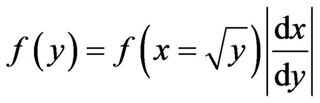 (8)
(8)
where 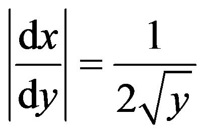 is the absolute value of the Jacobian of the transformation [15]. Thus
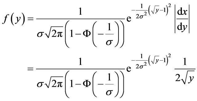
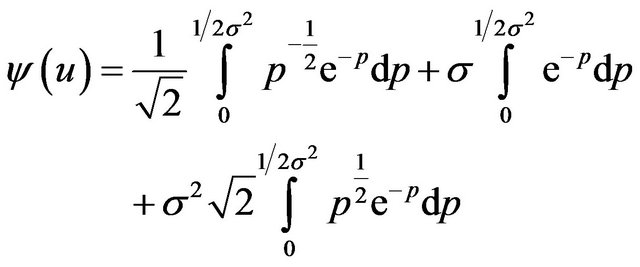
hence
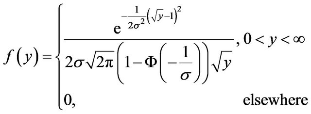 (9)
(9)
The crucial question is now “is (9) a proper pdf?”. If it is to be a proper pdf, it must satisfy the condition;
1) 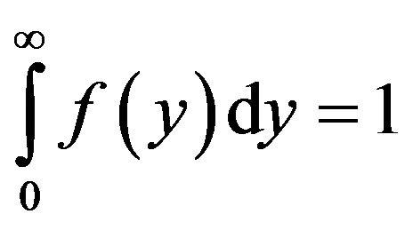
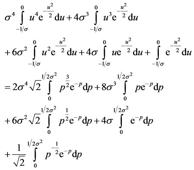
hence we now proceed to show that the integral of (9) is equal to unity as follows:
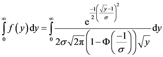 (10)
(10)
Let
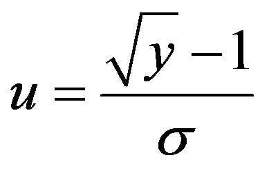 (11a)
(11a)
hence
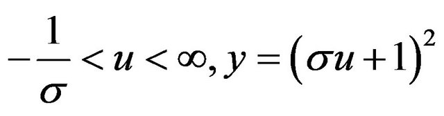 (11b)
(11b)
and
 (11c)
(11c)
therefore, substituting the results in (11a) through (11c) into (10) yields

and this shows that (9) is a proper pdf.
2.1. Mean of the Square Transformed Distribution, 
By definition
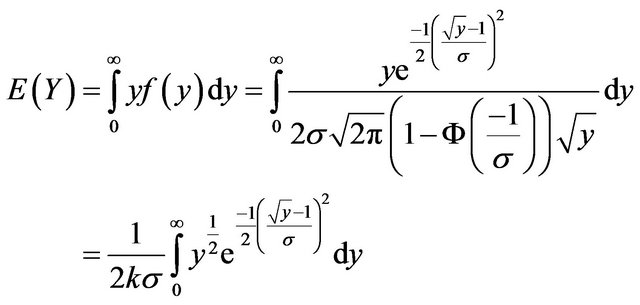 (12)
(12)
where
 .
.
Applying the substitution given in (11) into (12), we obtain
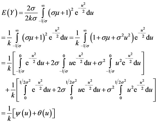 (13)
(13)
where
and
If we let
 (14)
(14)
in , we obtain
 (15a)
(15a)
and
 (15b)
(15b)
hence
 (16)
(16)
By integration by parts the following results are obtained
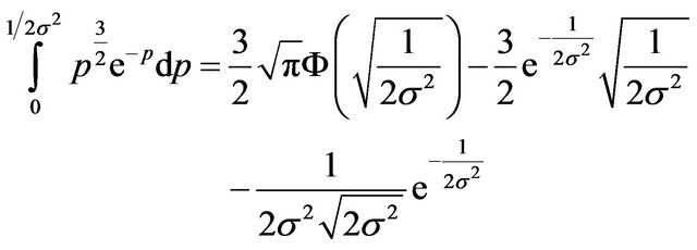 (17a)
(17a)
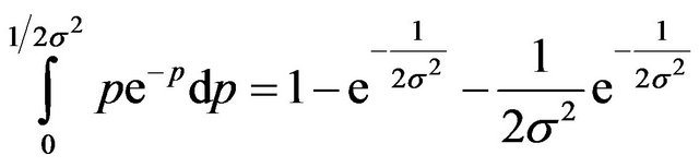 (17b)
(17b)
 (17c)
(17c)
 (17d)
(17d)
 (17e)
(17e)
hence
 (18)
(18)
Furthermore, if we let
 (19)
(19)
in , we obtain
 (20a)
(20a)
and
 (20b)
(20b)
thus
 (21)
(21)
Substituting the results of (18), (21) and the value of k into (13), we obtain
 (22)
(22)
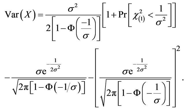
2.2. Variance of the Square Transformed Distribution ,
, 
By definition
 but
but
 (23)
(23)
Applying the transformation given in (11) into (23), we have that
 (24)
(24)
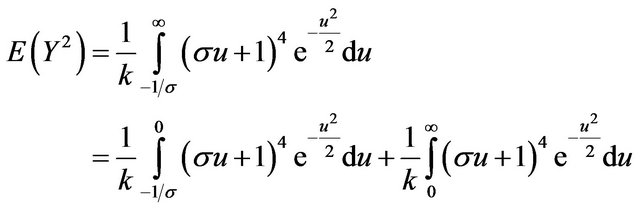
But
 (25)
(25)
and
 (26)
(26)
Applying the substitution in (14) and its corresponding results in (15) into (26), we have that
 (27)
(27)
Using the results given in (17), it can be shown after a series of algebraic manipulations, that (27) is equal to
 (28)
(28)
hence
 (29)
(29)
Furthermore applying the substitution in (19) and its corresponding results in (20a) and (20b) into
 , we obtain
 (30)
(30)
Substituting the results in (29) and (30) and the value of k into (24), we have that
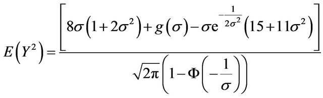 (31)
(31)
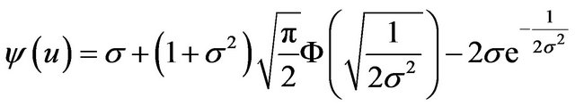
where
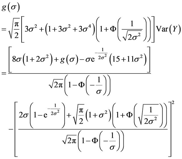 (32)
(32)
3. Condition for Successful Square Transformation
In this section, the interval  for which the desirable properties of the square transformed left-truncated
  distribution is approximately the same to that of the untransformed. The properties of interest are unit mean and normality and as a result we would first determine the interval
  for which the means of the transformed and the untransformed distributions of interest are both equal to unity (That is
 ). Secondly we would determine the
Table 1. An abridged table showing the computations of E(X), E(Y), Var(X) and Var(Y).

value of  for which the curve shapes of the two probability distributions are bell-shaped and symmetrical about a unit mean.
For the purpose of this investigation,  ,
,  and
and  using Equations (3), (4), (22) and (32) are computed for values of
 ,
, . The results of the computations are given in Table 1 (For want of space, Table 1 is an abridged table). From Table 1, the following results are true;
1)  to one decimal place (dp) for the interval
 .
.
2)  to two decimal places for the interval
 . In order to determine the number of decimal place(s) to use, we investigate the normality of the pdf curves of the square transformed and that of the untransformed distributions at the points b = 0.027 and 0.280. The investigation of normality at the two points is based on the previous studies of [1,12,13] whereby, normality of a pdf curve at a point b implied normality at points
 . Bell-shaped curves and symmetry about a unit mean would be a measure of normality. The pdf curves of the two distributions of interest for b = 0.027, 0.280 are given in Figures 1 and 2.
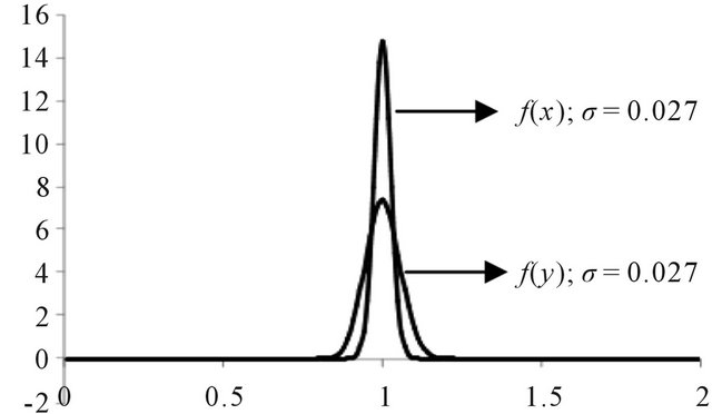
Figure 1. Curve Shapes of the Square-transformed  and Untransformed
  probability density function of the left-truncated
  Distribution for
 .
.
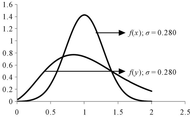
Figure 2. Curve Shapes of the Square-transformed  and Untransformed
  probability density function of the left-truncated
  Distribution for
 .
.
From the Figures, it is obvious that there is a clear departure from normality for the pdf curves for b = 0.280, therefore the acceptable interval is , since there is clear evidence of normality at b = 0.027. It is also clear from Table 1 that
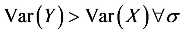 . Furthermore it is also evidenced from Table 1 that
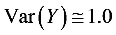 ,
,  , hence
 ,
,  correct to one decimal place (dp).
4. Summary and Conclusion
In this study we have established the pdf of the square transformed left-truncated  error component of the multiplicative time series model and the functional expressions for its mean and variance. Furthermore the mean and variance of the square transformed left-truncated
  error component and those of the untransformed component were compared for the purpose of establishing the interval for σ where the properties of the two distributions are approximately the same in terms of equality of means and normality. From the results of the study, it was established that the two distributions are normally distributed and have means
  correct to 1dp in the interval
 .
.
Based on the results of this study we therefore conclude that successful square transformation where necessary is achieved for values of σ such that . However caution has to be exercised since square transformation leads to increased error variance.
REFERENCES
- I. S. Iwueze, “Some Implications of Truncating the N (1, s2) Distribution to the Left at Zero,” Journal of Applied Sciences, Vol. 7, No. 2, 2007, pp. 189-195. doi:10.3923/jas.2007.189.195
- C. Chatfield, “The Analysis of Time Series: An Introduction,” Chapman and Hall, CRC Press, Boca Raton, 2004.
- D. B. Percival and A. T. Walden, “Wavelet Methods for Time Series Analysis,” Cambridge University Press, Cambridge, 2000.
- M. B. Priestley, “Spectral Analysis and Time Series Analysis,” Vol. 1-2, Academic Press, London, 1981.
- G. E. P. Box, G. M Jenkins and G. C. Reinsel, “Time Series Analysis, Forecasting and Control,” 3rd Edition, Prentice-Hall, Englewood Cliffs, 1994.
- W. W. Wei, “Time Series Analysis: Univariate and Multivariate Methods,” Addison-Wesley Publishing Company, Inc., Redwood City, 1989.
- M. G. Kendal and J. K. Ord, “Time Series,” 3rd Edition, Charles Griffin, London, 1990.
- I. S. Iwueze, E. C. Nwogu, J. Ohakwe and J. C. Ajaraogu, “Uses of the Buys-Ballot Table in Time Series Analysis,” Applied Mathematics, Vol. 2, No. 5, 2011, pp. 633-645. doi:10.4236/am.2011.25084
- M. S. Bartlett, “The Use of Transformations,” Biometrica, Vol. 3, No. 1, 1947, pp. 39-52. doi:10.2307/3001536
- G. E. P. Box and D. R. Cox, “An Analysis of Transformations,” Journal of the Royal Statistical Society, Series B, Vol. 26, No. 2, 1964, pp. 211-243.
- A. C. Akpanta and I. S. Iwueze, “On Applying the Bartlett Transformation Method to Time Series Data,” Journal of Mathematical Sciences, Vol. 20, No. 3, 2009, pp. 227-243.
- C. R. Nwosu, I. S. Iwueze and J. Ohakwe, “Distribution of the Error Term of the Multiplicative Time Series Model under Inverse Transformation,” Advances and Applications in Mathematical Sciences, Vol. 7, No. 2, 2010, pp. 119-139.
- E. L. Otuonye, I. S. Iwueze and J. Ohakwe, “The Effect of Square Root Transformation on the Error Component of the Multiplicative Time Series Model,” International Journal of Statistics and Systems, Vol. 6, No. 4, 2011, pp. 461-476.
- J. Ohakwe, O. A. Dike and A. C. Akpanta, “The Implication of Square Root Transformation on a Gamma Distributed Error Component of a Multiplicative Time Series Model,” Proceedings of African Regional Conference on Sustainable Development, Vol. 6, No. 4, 2012, pp. 65-78.
- R. V. Hogg and A. T. Craig, “Introduction to Mathematical Statistics,” 6th Edition, Macmillan Publishing Co. Inc., New York, 1978.
NOTES
*Corresponding author.