Applied Mathematics
Vol.4 No.6(2013), Article ID:33152,12 pages DOI:10.4236/am.2013.46129
Exponential B-Spline Solution of Convection-Diffusion Equations
Department of Mathematics, University of Neyshabur, Neyshabur, Iran
Email: rez.mohammadi@gmail.com
Copyright © 2013 Reza Mohammadi. This is an open access article distributed under the Creative Commons Attribution License, which permits unrestricted use, distribution, and reproduction in any medium, provided the original work is properly cited.
Received September 25, 2012; revised April 21, 2013; accepted April 30, 2013
Keywords: Exponential B-Spline; Convection-Diffusion Equation; Collocation; Crank-Nicolson Formulation; Unconditionally Stable
ABSTRACT
We present an exponential B-spline collocation method for solving convection-diffusion equation with Dirichlet’s type boundary conditions. The method is based on the Crank-Nicolson formulation for time integration and exponential B-spline functions for space integration. Using the Von Neumann method, the proposed method is shown to be unconditionally stable. Numerical experiments have been conducted to demonstrate the accuracy of the current algorithm with relatively minimal computational effort. The results showed that use of the present approach in the simulation is very applicable for the solution of convection-diffusion equation. The current results are also seen to be more accurate than some results given in the literature. The proposed algorithm is seen to be very good alternatives to existing approaches for such physical applications.
1. Introduction
Convection-diffusion equation plays an important role in the modeling of several physical phenomena where energy is transformed inside a physical system due to two processes: convection and diffusion. The term convection means the movement of molecules within fluids, whereas, diffusion describes the spread of particles through random motion from regions of higher concentration to regions of lower concentration. Also this equation describes advection-diffusion of quantities such as heat, energy, mass, etc. They find their applications in water transfer in soils, heat transfer in draining film, spread of pollutants in rivers, dispersion of tracers in porous media. They are also widely used in studying the spread of solute in a liquid flowing through a tube, long range transport of pollutants in the atmosphere, flow in porous media and many others [1-4].
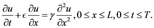
We consider the initial-value problem for the one-dimensional time-dependent convection-diffusion equation
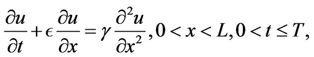 (1)
(1)
subjected to the initial conditions
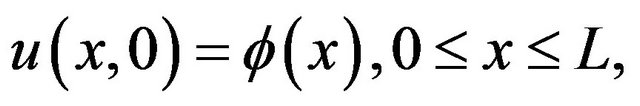 (2)
(2)
and with appropriate Dirichlet boundary conditions
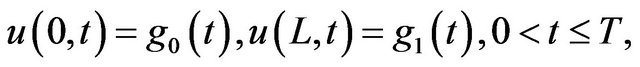 (3)
(3)
where the parameter  is the viscosity coefficient and
  is the phase speed and both are assumed to be positive.
  and
and  are known functions with sufficient smoothness.
It is necessary to calculate the transport of fluid properties or trace constituent concentrations within a fluid for applications such as water quality modeling, air pollution, meteorology, oceanography and other physical sciences. When velocity field is complex, changing in time and transport process cannot be analytically calculated, and then numerical approximations to the convection equation are indispensable [4]. They are also important in many branches of engineering and applied science. Therefore many researchers have spent a great deal of effort to compute the solution of these equations using various numerical methods. There are many studies on the numerical solution of initial and initial-boundary problems of convection-diffusion equation [1,3-24] include finite difference methods, Galerkin methods, spectral methods, wavelet-based finite elements, B-spline methods and several others. These equations are characterized by no dissipative advective transport component and a dissipative diffusive component. When diffusion is the dominant factor, aall numerical profiles go well. On the contrary, most numerical results exhibit some combination of spurious oscillations and excessive numerical diffusion, when advection is dominant transport process. These behaviors can be easily explained using a general Fourier analysis, little progress has been made to overcome such difficulties effectively. Using extremely fine mesh is one such alternative but is not prudent to apply it as it is computationally costlier. So a great effort has been made on developing the efficient and stable numerical techniques.
Nguyen and Reynen [5] presented a space-time leastsquares finite-element scheme for advection-diffusion equation. Codina [7] considered several finite-element methods for solving the diffusion-convection-reaction equation and showed that Taylor-Galerkin method has a stabilization effect similar to a sub grid scale model, which is in turn related to the introduction of bubble functions. Dehghan [12] developed several different numerical techniques for solving the three-dimensional advection-diffusion equation with constant coefficients and compared them with other methods in literature. These techniques are based on the two-level fully explicit and fully implicit finite difference approximations. Dehghan [13] developed a new practical scheme designing approach whose application is based on the modified equivalent partial differential equation (MEPDE). Dehghan and Mohebbi [20] presented new classes of high-order accurate methods for solving the two-dimensional unsteady convection-diffusion equation based on the method of lines approach. These methods are second-order accurate and techniques that are third order or fourth order accurate. Dehghan [14] derived a variety of explicit and implicit algorithms based on the weighted finite difference approximations dealing with the solution of the one-dimensional advection equation. Dehghan and Shakeri [21] obtained the solution of Cauchy reaction-diffusion problem via variational iteration method.
It is well-known that a good interpolating or approximating scheme, in addition to the standard requests as good approximation rate, low computational cost, numerical reliability, should possess the capability of reproducing the shape of the data. It has been found in the literature that using piecewise polynomial functions leads to better convergence results and simpler proofs than using polynomials. Recently, Spline and B-spline functions together with some numerical techniques have been used in getting the numerical solution of the differential equations. Kadalbajoo and Arora [4] used Taylor-Galerkin methods together with the type of splines known as Bsplines to construct the approximation functions over the finite elements for the solution of time-dependent advection-diffusion problems. Mittal and Jain [1] discussed collocation method based on redefined cubic B-splines basis functions for solving convection-diffusion equation with Dirichlet’s type boundary conditions. The main objective of this study is to develop a user friendly, economical and stable method which can work for higher values of Péclet number for convection-diffusion equation by using redefined cubic B-splines collocation method.
In the current paper, we develop the collocation method by using the exponential B-spline function for numerical solution of the convection-diffusion equation. Our main aim is to improve the accuracy of B-spline method by involving some parameters, which enable us to obtain the classes of methods. Our method is a modification of cubic B-spline method for solution of (1). Application of our method is simple and in comparison with the existing well-known methods is accurate. While solving initial boundary value problems in partial differential equations, the procedure is to combine a spline approximation for the space derivative with a Crank-Nicolson finite difference approximation for the time derivative. The combination of a finite difference and an exponential spline function techniques provide better accuracy than the finite difference methods. Therefore, the time derivative is replaced by finite difference representation and the first-order space and second-order space derivatives by exponential B-spline. Also, we study stability for the new method and will show that it is unconditionally stable. We use the exponential B-splines basis that leads to the tri-diagonal system which can be solved by the well known algorithm. Numerical examples are presented which demonstrate that the present scheme with exponential B-splines gives more accurate approximations than the scheme using cubic B-splines. Similar to the method in [1] our method is a user friendly, economical and stable method which can work for higher values of Péclet number for convection-diffusion equation.
This paper is arranged as follows. In Section 2, the Bsplines basis for the space of exponential spline is given and some interpolation results for the exponential spline interpolate are stated. In Section 3, the construction of the exponential B-spline collocation method for the solution of the convection-diffusion equation is described. The stability analysis of the presented method is discussed in Section 4. In Section 5, numerical experiments are conducted to demonstrate the efficiency of the proposed method and confirm it’s theoretical behavior. These computational results show that our proposed algorithm is effective and accurate in comparison with the literature. Finally results of experiments and the conclusions are included in Section 7.
Let  denotes the value of
  at the nodal points
 , that is,
 . Then we use
 in the remaining parts of the paper.
2. Exponential Spline Functions
Let  be the given interval and
  be the partition of
  defined as
 , with mesh spacing
 . The function
  is said to be a cubic spline over
  if
if  and
and  restricted to
  is a cubic polynomial for
  .
.
The cubic spline  is well known to have the following analogue in the beam theory. Consider a simply supported beam with supports
 .
.
Then , the deflection of the beam, is a solution to the differential equation
 , for
, for
 . Here E = Young’s modulus, I = Crosssectional moment of inertia, M = Bending moment and
  denotes the second order differential operator. Differentiating the above equation twice, we obtain the following two point boundary value problems on each subinterval
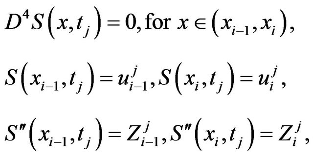 (4)
(4)
where  and
and  are uniquely determined from the condition
 , for given
  and
and . Here
  is the fourth order differential operator.
The cubic spline  so defined has a tendency to exhibit unwanted undulations. The above analogy suggests that the application of the uniform tension between the supports might be a remedy to the problem. Then the beam equation becomes
 for
for . Let
. Let ![]() be the set of tension parameters defined on each subinterval
be the set of tension parameters defined on each subinterval .
.
Suppose , then the above consideration leads to define the exponential spline
  as the solution to the boundary value problems on each subinterval
 .
.
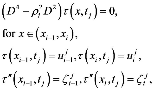 (5)
(5)
with  yet to be determined. Note that
  implies that
 ,
,  , which gives the cubic splines; while
  implies that
 ,
,  , which gives the linear splines.
Following [25,26] the solution of the above boundary value problem is
 (6)
(6)
where  s are prescribed non-negative real numbers and
  is an exponential spline of order four, lies in the
 .
.
Thus in general we can define the exponential spline of order  as the function
  whose restriction on non-empty interval
 , for
, for
 , lies in the
 .
.
Among the various classes of splines, the polynomial spline has been received the greatest attention primarily because it admits a basis of B-splines which can be accurately and efficiently computed. It has been shown that the exponential spline also admits a basis of Bsplines which can be defined as follows. Let  be the B-spline centered at
  and having a finite support on the four consecutive intervals
 .
.
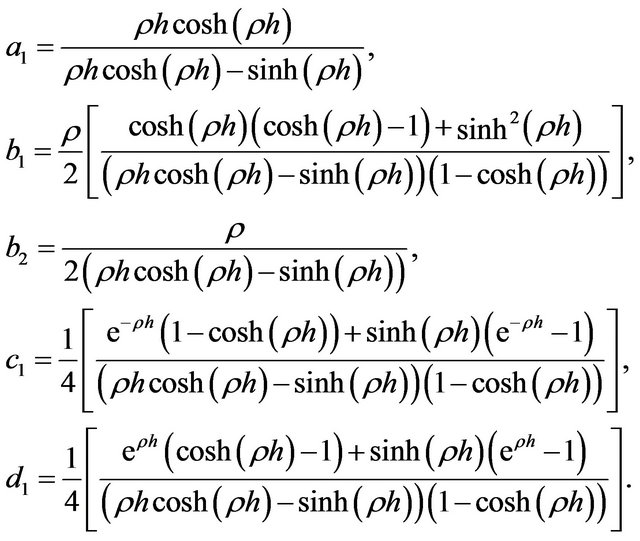
According to McCartin [27], the  can be defined as
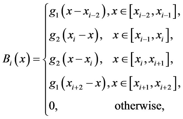 (7)
(7)
where
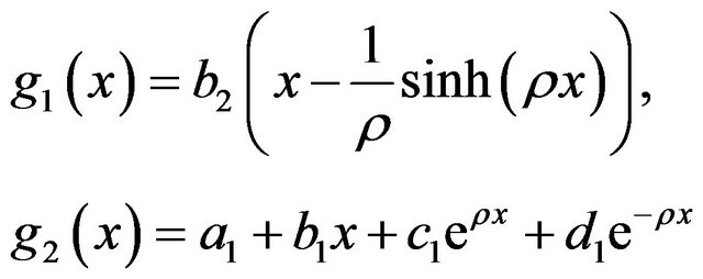
and
Each basis function  is twice continuously differentiable. The values of
  and
and  at the nodal points
  ‘s are shown in Table 1.
Let  be the cubic spline and
  be the exponential spline. Now we consider to the following results which have been established by Pruess [28].
Theorem 2.1
Similar to the above theorem we have another companion result due to McCartin [29].
Theorem 2.2

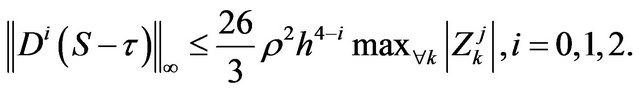
These theorems together with the de Boor-Hall error estimate Prenter leads to the following corollary.
Corollary 2.1 If  then there exits a constant,
  , independent of
  such that
![]()
3. Numerical Method
The region  is partitioned into n finite elements of equal length h by knots
 , such that
 . Let
. Let  be the exponential B-splines with both knots
  and 2 additional knots outside the region, positioned at:
The set of exponential B-splines  forms a basis for functions defined over the problem domain
 . The exponential B-splines (Equation (7)) and it’s first and second derivatives vanish outside the interval
 .
.
An approximate solution  to the analytical solution
  will be sought in form of an expansion of B-splines:
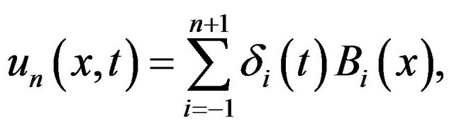 (8)
(8)
where  are time dependent parameters to be determined from the exponential B-spline collocation form of Equation (1).
Using the expression (8) and Table 1, nodal value ![]() and its first and second derivatives at the knots
and its first and second derivatives at the knots  are obtained in terms of the element parameters by:
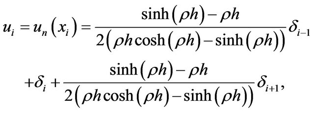 (9)
(9)
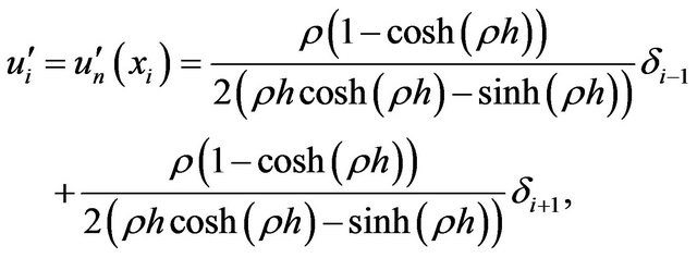 (10)
(10)
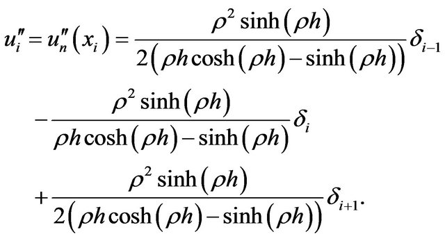 (11)
(11)
To apply the proposed method, discretizing the time derivative in the usual finite difference way and applying
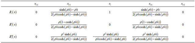
Table 1. Exponential B-spline basis values.
Crank-Nicolson scheme to (1), we get
 (12)
(12)
where  is the time step.
Substituting the approximate solution  for
for ![]() and putting the values of the nodal values
and putting the values of the nodal values , its derivatives using Equations (9)-(11) at the knots in Equation (12) yields the following difference equation with the variables
![]() ,
,
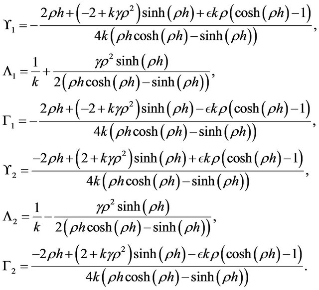
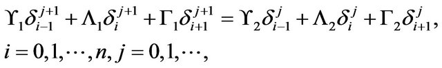 (13)
(13)
where
The system (13) consists of  linear equations in of
  unknowns
To obtain a unique solution to this system two additional constraints are required. These are obtained from the boundary conditions. Imposition of the boundary conditions enables us to eliminate the parameters  and
and  from the system. Eliminating
  and
and , the system (13) is reduced to a tri-diagonal system of
  linear equations with
  unknowns. This tri-diagonal system can be solved by Thomas algorithm.
The time evolution of the approximate solution  is determined by the time evolution of the vector
  which is found repeatedly by solving the recurrence relation, once the initial vectors
  have been computed from the initial and boundary conditions.
3.1. Treatment of Boundary Conditions
In order to eliminate the parameters  and
and  from the system we have used the boundary conditions (3).
From (3) we have
Expanding ![]() in terms of approximate exponential B-spline formula from (9) at
in terms of approximate exponential B-spline formula from (9) at  putting
  in (9), we get
 (14)
(14)
Similarly at  putting
  in (9) we get
 (15)
(15)
Solving the obtained equations we get the values of  in terms of
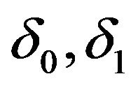 . Similarly
  can be expressed in terms of
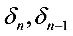 .
.
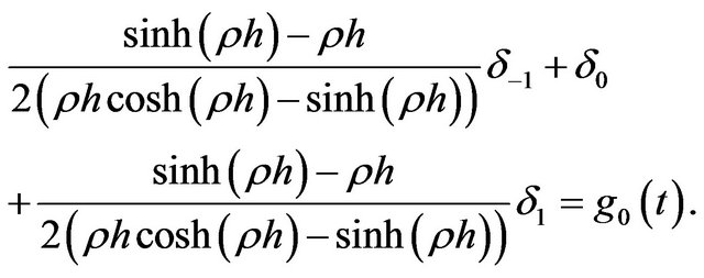
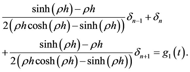
3.2. The Initial State
The initial vector  can be determined from the initial condition
 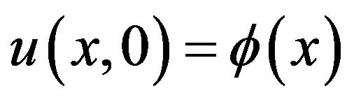 which gives
  equation in
  unknowns. For the determination of the unknowns relations at the knot are used
4. Stability Analysis
We have investigated stability of the presented method by applying von-Neumann method. Now, we cosider the trial solution (on Fourier mode out of the full solution) at a given point 
 (16)
(16)
where β the mode number, h is the element size and .
.
Now, by substituting (16) in (13), and symlifying the equation, we obtain
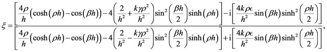 (17)
(17)
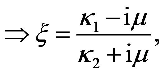 (18)
(18)
where
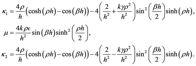
Following [1], by substituting 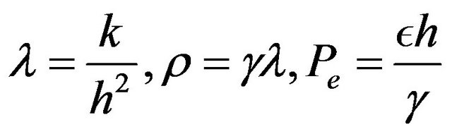 and
and , where Pe is called Péclet number in (18)we get
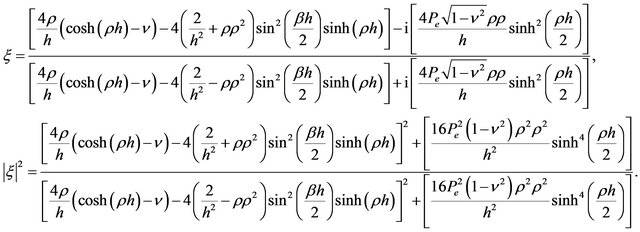 (19)
(19)
Since numerator in (19) is less than denominator, therefore , hence the method is unconditionally stable. It means that there is no restriction on the grid size, i.e. on
  and
and , but we should choose them in such a way that the accuracy of the scheme is not degraded.
5. Numerical Illustrations
In this section, some numerical examples are presented to evaluate the performance of the proposed method. We consider six convection-diffusion equations which the exact solutions are known to us. To illustrate our presented method and to demonstrate it’s applicability computationally, computed solutions for different values of  and
and  are compared with exact solutions at grid points and with the results in existing methods. All programs are run in Mathematica 6.0. The computed absolute errors and maxsimume absolute errors in numerical solutions are listed in Tables.
For the sake of comparison, following [1], some important non-dimensional parameters in numerical analysis are defined as follows:
Courant number: The Courant number is defined as
 .
.
Diffusion Number: The diffusion number is defined as .
.
Grid Péclet Number: The Péclet number is defined as
 .
.
Numerical results confirm that the Péclet number is high, the convection term dominates and when the Péclet number is low the diffusion term dominates.
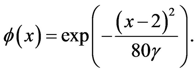
Example 5.1 Consider the convection-diffusion equation [1,10]

with  and subject to the initial conditions
The theoritical solution of this problem is

The boundary conditions are obtained from the theoritical solution.
In all computations, we take  α = 1.17712434446770, β = −0.09, h = 0.01 and k = 0.001, so that
  and
and . The absolute errors are tabulated in Tables 2 and 3 for different time levels. We observe that our presented method is more accurate in comparison with Mittal and Jain [1] and Douglas methods but less accurate to Ismail et al. [10] method. However, It is evident that our method is unconditionally stable while the method in [10] is conditionally stable.
Example 5.2 Consider the convection-diffusion equation [1,10]

with and subject to the initial conditions

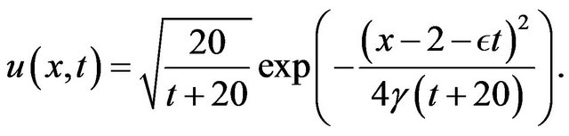
The analytical solution of this problem is
The boundary conditions are obtained from the analytical solution.
In all computations, we take 
 and k = 0.001, so that
  and
and . The absolute errors for different time levels are listed in Tables 4 and 5. We observe that our presented method is more accurate in comparison with existing methods. Also, for higher value of
  our method produces more accurate results in comparison with well known methods.
Example 5.3 Consider the following equation [1,3]

subjected to the following initial condition
The theoritical solution of this problem is
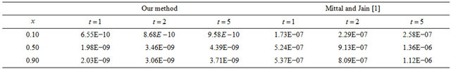
Table 2. The absolute errors of our method and the method in [1] for example 5.1.
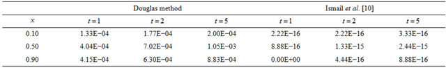
Table 3. The absolute errors of Douglas method and Ismail et al. [10] method for example 5.1.
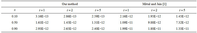
Table 4. The absolute errors of our method and the method in [1] for example 5.2.
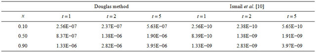
Table 5. The absolute errors of Douglas method and Ismail et al. [10] method for example 5.2.
The boundary conditions are obtained from the theoritical solution.
In all computations, we take 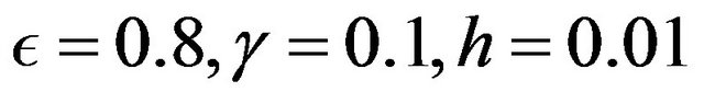 and k = 0.001, so that
 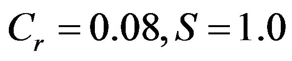 and
and . The absolute errors for different time levels are tabulated in Table 6. The results indicate that the errors in our method more or less is similar to [1] and [3] for t = 1, t = 2 and
  respectively, but the errors in our method for
 ![]() are much less than [3].
are much less than [3].
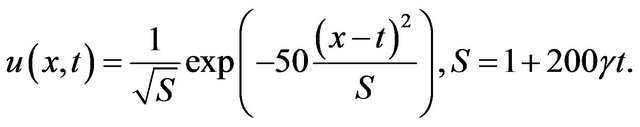
Example 5.4 Consider the following equation [1,4,6, 24]
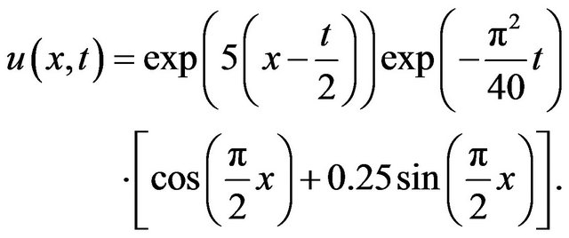
The analytical solution of this problem is
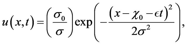
where  and subjected to the following initial condition
The boundary conditions are obtained from the analytical solution.
In this example, first similar to [24] we take L = 1,  and k = 0.001, so that
  and
and  The absolute errors for different time levels are tabulated in Table 7 and compared with results in [1]. The results indicate that the errors in our method more or less is similar to [1]. Then we compare our method with the methods in [1,4] in Table 8 where
  and
and![]() , so that
, so that . The results show that our method is considerably accurate in comparison with the methods in [1,4]. Following [1] we comput numerical solution at
  and
and  with
with  and
and , so that
 . The absolute errors are tabulated in Table 9 and compared with results in [1] which are listed in Table 10. The Tables show that our method is stable beside this our method is accurate in comparison with the method in [1].
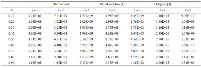
Table 6. The absolute errors of our method and the methods in [1,3] for example 5.3.
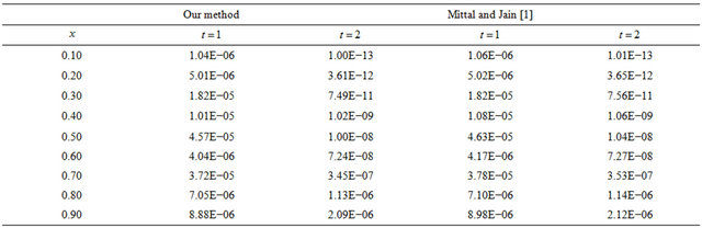
Table 7. The absolute errors of our method and the method in [1] for example 5.4 (with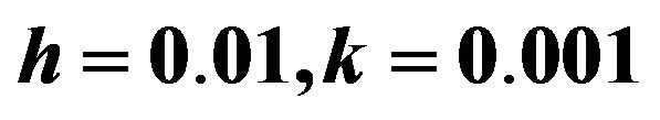 ).
).
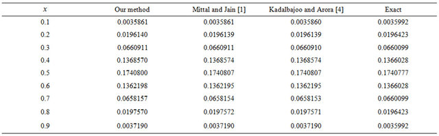
Table 8. Approximate and exact solutions for example 5.4 (with h = 0.01, k = 0.01 and t = 1.0).
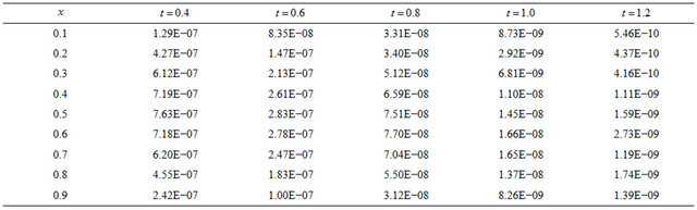
Table 9. The absolute errors of our method for example 5.4.
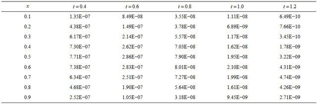
Table 10. The absolute errors of the method in [1] for example 5.4.
For the sake of comparison with Mittal, we compute numerical solution at t = 1, 2, 3, 4, 5 and  with
with  and
and , so that
  and
and . The observed results are listed in Table 11 and compared with [1] in Table 12. The numerical approximations seem to be in good agreement with the exact solutions. Morever, the results indicate that our method is accurate in comparison with the method in [1].
Example 5.5 Consider the following equation [1,9]
with  subjected to the following initial condition
The theoritical solution of this problem is
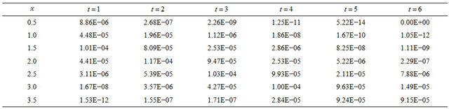
Table 11. The absolute errors of our method for example 5.4.
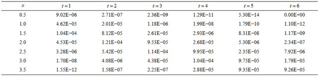
Table 12. The absolute errors of the method in [1] for example 5.4.
The boundary conditions are obtained from the theoritical solution.
We compute maximum absolute errors with 
 , so that
 . The results are computed for different time levels and listed in Table 13. Also we compare our results with the results in [1,9]. The results indicate that the errors in our method more or less is similar to [1] but the errors in our method are much less than the errors in [9].
Example 5.6 Consider the following equation [1,23]

with  and subjected to the following initial condition
The analytical solution of this problem is
The boundary conditions are obtained from the analytical solution.
We compute maximum absolute errors with 
 and
and , so that
 . The observed results are tabulated in Table 14 and compared with results in [1,23]. This results show that our method is considerable accurate in compare with the methods in [1,23].
6. Discussions
In this article, an exponential B-spline scheme has been proposed to solve the convection-diffusion equation with Dirichlet’s type boundary conditions and has been efficiently illustrated. To tackle this, the proposed scheme of exponential B-spline in space and the Crank-Nicolson scheme in time have been combined. By taking different values of parameter  we can obtain various classes of methods. But in all computations we choose
  which is the optimum case of our method. Stability of this method has been discussed and shown that it is unconditionally stable. The performance of the current scheme for the problem has been measured by comparing with the exact solutions. For comparison purposes, the results of the scheme are exhibited for various values of the corresponding parameters. Comparisons of the computed results with exact solutions showed that the scheme is capable of solving the convection-diffusion equation and producing highly accurate solutions with minimal computational effort. It was seen that the proposed scheme approximate the exact solution very well. The produced results were seen to be more accurate than

Table 13. Maximum absolute errors for example 5.5.
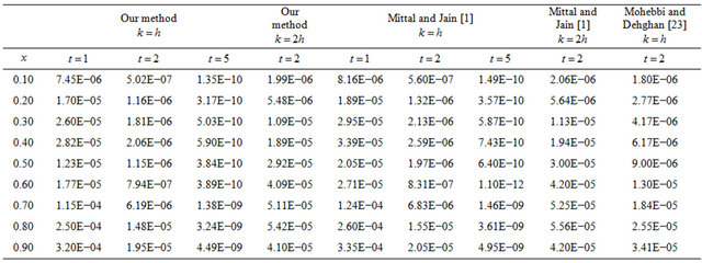
Table 14. Absolute errors for example 5.6 with h = 0.01.
some available results given in the literature. This technique has been seen to be very good alternative to some existing ones in solving physical problems represented by the nonlinear partial differential equations.
REFERENCES
- R. C. Mittal and R. K. Jain, “Redefined Cubic B-Splines Collocation Method for Solving Convection-Diffusion Equations,” Applied Mathematical Modelling, 2012, in Press. doi:10.1016/j.apm.2012.01.009
- M. A. Celia, T. F. Russell, I. Herrera and R. E. Ewing, “An Eulerian-Langrangian Localized Adjoint Method for the Advection-Diffusion Equation,” Advances in Water Resources, Vol. 13, No. 4, 1990, pp. 187-206. doi:10.1016/0309-1708(90)90041-2
- M. Dehgan, “Weighted Finite Difference Techniques for the One-Dimensional Advection Diffusion Equation,” Applied Mathematics and Computation, Vol. 147, No. 2, 2004, pp. 307-319. doi:10.1016/S0096-3003(02)00667-7
- M. K. Kadalbajoo and P. Arora, “Taylor-Galerkin BSpline Finite Element Method for the One-Dimensional Advection-Diffusion Equation,” Numerical Methods for Partial Differential Equations, Vol. 26, No. 5, 2010, pp. 1206-1223.
- H. Nguyen and J. Reynen, “A Space Time Least-Squares Finite-Element Scheme for Advection-Diffusion Equation,” Computer Methods in Applied Mechanics and Engineering, Vol. 42, 1984, pp. 331-442. doi:10.1016/0045-7825(84)90012-4
- Rizwan-Uddin, “A Second-Order Space and Time Nodal Method for the One-Dimensional Convection-Diffusion Equation,” Computers & Fluids, Vol. 26, No. 3, 1997, pp. 233-247. doi:10.1016/S0045-7930(96)00039-4
- R. Codina, “Comparison of Some Finite-Element Methods for Solving the Diffusion-Convection-Reaction Equation,” Computer Methods in Applied Mechanics and Engineering, Vol. 156, No. 1, 1998, pp. 185-210. doi:10.1016/S0045-7825(97)00206-5
- M. M. Chawla, M. A. Al-Zanaidi and D. J. Evans, “Generalized Trapezoidal Formulas for Convection-Diffusion Equations,” International Journal of Computer Mathematics, Vol. 72, No. 2, 1999, pp. 141-154. doi:10.1080/00207169908804841
- M. M. Chawla, M. A. Al-Zanaidi and M. G. Al-Aslab, “Extended One Step Time-Integration Schemes for Convection-Diffusion Equations,” Computers & Mathematics with Applications, Vol. 39, No. 3-4, 2000, pp. 71-84. doi:10.1016/S0898-1221(99)00334-X
- H. N. A. Ismail, E. M. E. Elbarbary and G. S. E. Salem, “Restrictive Taylor’s Approximation for Solving Convection-Diffusion Equation,” Applied Mathematics and Computation, Vol. 147, No. 2, 2004, pp. 355-363. doi:10.1016/S0096-3003(02)00672-0
- S. Karaa and J. Zhang, “High Order ADI Method for Solving Unsteady Convection-Diffusion Problems,” Journal of Computational Physics, Vol. 198, No. 1, 2004, pp. 1-9. doi:10.1016/j.jcp.2004.01.002
- M. Dehghan, “Numerical Solution of the Three-Dimensional Advection-Diffusion Equation,” Applied Mathematics and Computation, Vol. 150, No. 1, 2004, pp. 5-19. doi:10.1016/S0096-3003(03)00193-0
- M. Dehghan, “On the Numerical Solution of the OneDimensional Convection-Diffusion Equation,” Mathematical Problems in Engineering, Vol. 2005, No. 1, 2005, pp. 61-74. doi:10.1155/MPE.2005.61
- M. Dehghan, “Quasi-Implicit and Two-Level Explicit Finite-Difference Procedures for Solving the One-Dimensional Advection Equation,” Applied Mathematics and Computation, Vol. 167, No. 1, 2005, pp. 46-67. doi:10.1016/j.amc.2004.06.067
- D. K. Salkuyeh, “On the Finite Difference Approximation to the Convection-Diffusion Equation,” Applied Mathematics and Computation, Vol. 179, No. 1, 2006, pp. 79- 86. doi:10.1016/j.amc.2005.11.078
- I. Dag, D. Irk and M. Tombul, “Least-Squares Finite-Element Method for the Advection-Diffusion Equation,” Applied Mathematics and Computation, Vol. 173, No. 1, 2006, pp. 554-565. doi:10.1016/j.amc.2005.04.054
- H. Karahan, “Implicit Finite Difference Techniques for the Advection-Diffusion Equation Using Spreadsheets,” Advances in Engineering Software, Vol. 37, No. 9, 2006, pp. 601-608. doi:10.1016/j.advengsoft.2006.01.003
- H. Karahan, “A Third-Order Upwind Scheme for the Advection-Diffusion Equation Using Spreadsheets,” Advances in Engineering Software, Vol. 38, No. 10, 2007, pp. 688-697. doi:10.1016/j.advengsoft.2006.10.006
- H. Karahan, “Unconditional Stable Explicit Finite Difference Technique for the Advection-Diffusion Equation Using Spreadsheets,” Advances in Engineering Software, Vol. 38, No. 2, 2007, pp. 80-86. doi:10.1016/j.advengsoft.2006.08.001
- M. Dehghan and A. Mohebbi, “High-Order Compact Boundary Value Method for the Solution of Unsteady Convection-Diffusion Problems,” Mathematics and Computers in Simulation, Vol. 79, No. 3, 2008, pp. 683-699. doi:10.1016/j.matcom.2008.04.015
- M. Dehghan and F. Shakeri, “Application of He’s Variational Iteration Method for Solving the Cauchy ReactionDiffusion Problem,” Journal of Computational and Applied Mathematics, Vol. 214, No. 2, 2008, pp. 435-446. doi:10.1016/j.cam.2007.03.006
- H. F. Ding and Y. X. Zhang, “A New Difference Scheme with High Accuracy and Absolute Stability for Solving Convection-Diffusion Equations,” Journal of Computational and Applied Mathematics, Vol. 230, No. 2, 2009, pp. 600-606. doi:10.1016/j.cam.2008.12.015
- A. Mohebbi and M. Dehghan, “High-Order Compact Solution of the One-Dimensional Heat and AdvectionDiffusion Equations,” Applied Mathematical Modelling, Vol. 34, No. 10, 2010, pp. 3071-3084. doi:10.1016/j.apm.2010.01.013
- M. Sari, G. Güraslan and A. Zeytinoglu, “High-Order Finite Difference Schemes for Solving the Advection-Diffusion Equation,” Computers & Mathematics with Applications, Vol. 15, No. 3, 2010, pp. 449-460.
- S. Chandra Sekhara Rao and M. Kumar, “Exponential BSpline Collocation Method for Self-Adjoint Singularly Perturbed Boundary Value Problems,” Applied Numerical Mathematics, Vol. 58, No. 10, 2008, pp. 1572-1581. doi:10.1016/j.apnum.2007.09.008
- S. Chandra Sekhara Rao and M. Kumar, “Parameter-Uniformly Convergent Exponential Spline Difference Scheme for Singularly Perturbed Semilinear Reaction-Diffusion Problems,” Nonlinear Analysis, Vol. 71, 2009, pp. 1579- 1588. doi:10.1016/j.na.2009.01.210
- B. J. Mc Cartin, “Theory of Exponential Splines,” Journal of Approximation Theory, Vol. 66, No. 1, 1991, pp. 1-23. doi:10.1016/0021-9045(91)90050-K
- S. Pruess, “Properties of Splines in Tension,” Journal of Approximation Theory, Vol. 17, No. 1, 1976, pp. 86-96. doi:10.1016/0021-9045(76)90113-1
- B. J. Mc Cartin, “Theory, Computation, and Application of Exponential Splines,” Courant Mathematics and Computing Laboratory Research and Development Report, DOE/ER/03077-171, 1981.