Applied Mathematics
Vol. 3 No. 11 (2012) , Article ID: 24511 , 9 pages DOI:10.4236/am.2012.311229
Optimal Campaign in Leptospirosis Epidemic by Multiple Control Variables
1Department of Mathematics, University of Malakand, Chakdara, Pakistan
2Department of Mathematics, Abdul Wali Khan University, Mardan, Pakistan
3Department of Business Administration and Accounting, Buraimi University College, Al-Buraimi, Oman
Email: gzaman@uom.edu.pk
Received August 17, 2012; revised September 28, 2012; accepted October 5, 2012
Keywords: Mathematical Model; Optimal Control; Pontryagin’s Maximum Principle; Numerical Results
ABSTRACT
In this paper, we consider a leptospirosis epidemic model to implement optimal campaign by using multiple control variables. First, we show the existence of the control problem. Then we derive the conditions under which it is optimal to eradicate the leptospirosis infection and examine the impact of a possible educatioal/vaccinaction campaign using Pontryagin’s Maximum Principle. We completely characterize the optimal control problem and compute the numerical solution of the optimality system using an iterative method. The results obtained from the numerical simulations of the model show that a possible educational/vaccinaction combined with effective treatment regime would reduce the spread of the leptospirosis infection appreciably.
1. Introduction
Leptospirosis disease is a globally zoonotic disease. The cause of the disease is bacteria which is called leptospira. Human as well as cattle are mostly infected from this disease. The human are infected by means of drinking the water in which a rat (dead) found, while cattle that drink this water are become infectious. The human whose urine is used by other animals and cattle are also infected, because the leptospirosis germs come out in urine. It is also reported that people belong to city are mostly infected from this disease and got liver infection. Leptospirosis is known by different names such Weil’s disease, canicola fever, canefield fever, 7-day fever, nanukayami fever [1]. Weil is the first man who credited that described leptospirosis as a unique disease process in 1886, 30 years before Inada and his colleagues identified the causal organism. The symptoms of leptospirosis are high fever, headache, chills, muscle aches, conjunctivitis (red eyes), diarrhea, vomiting, and kidney or liver problems (which may also include jaundice), anemia and sometimes rash. Symptoms may last from a few days and up to several weeks. Some reports also show that deaths from this disease may occur but they are rare. For somecases, the infections can be mild and without obvious symptom [2-6]. Outbreaks of this disease depending on season which often linked to environmental factors involve animals, agricultural and occupational cycles [7].
The mathematical formulation and dynamical sketch of this infection has been studied by several authors see for example [8-12]. Pongsuumpun et al. [11] represents mathematical model and considered some real data for numerical simulation. A simple deterministic model for the spread of leptospirosis in Thailand can be found in [13]. In their work, they represented the rate of change for both rats and human population. The human population is further divided into two main groups Juveniles and adults. Zaman [14] considered the real data presented in [13] to study the dynamical behavior and role of optimal control theory. The dynamical interaction between leptospirosis infected vector and human population is studied by Zaman et al. [12]. In their work, they presented global dynamics and bifurcation analysis. They also showed the numerical simulations for different values of the interaction parameter.
In case of vector born diseases some authors focused on eradication of the disease, by targeting the vector population as a strategy for controlling the disease [15, 16] while some scientists studied the effect of vaccinetion on the dynamics of the disease [14]. These scientists believed that optimal control theory is a powerful mathematical tools which make the decision involving complex dynamical systems [17]. Optimal control method has been used to study dynamics of the disease see for example [17-19]. Very little has been done in the interaction between leptospirosis infected vector and human population by applying multiple control variables to analyze and understand the dynamics of this infection in a community.
In this paper, we consider the basic model studied in [14] to incorporate some important epidemiological features and control functions. To control the spread of leptospirosis infection and the interaction of human with vector population, we use optimal theory to reduce the proportion of the infected human and infected vector until the disease cannot survive. At the long-term level of infected human by the interaction of infected vector which causes the spread of new infection. Therefore, if we can reduce the number of infected human further, so the disease does less well and will increase the recovered human. To do this, we introduce an educational/vaccinaction campaign by using three control variables. Our first control variable represents cover all cuts, water dry, full-cover boots, shoes and long sleeve shirts when handling animals, second control variable represents wash hands thoroughly on a regular basis and shower after work and third control variable represents clean up both work place and home. We first show the existence of the optimal control system. Then, we derive the conditions under which it is optimal to eradicate the leptospirosis infection and examine the impact of a possible educational/vaccinaction campaign using Pontryagin’s Maximum Principle. We also solve the optimality system numerically, which consists of the original state system, the adjoint system and their boundary conditions by using the data presented for leptospirosis epidemic in Thailand. We conclude by discussing results of the numerical simulations in detail.
The structure of the paper is organized as follows. Section 2 is devoted to the formulation of the basic mathematic model. In Section 3, we present the control problem and develop reproductive number. In Section 4, we present the endemic equilibria for both systems with and without control and bifurcation analysis. In Section 5, we present the existence of the control problem and derive the necessary conditions for an optimal control and the corresponding state system by using Pontryagin’s Maximum Principle. Section 6 is devoted to numerical solution of the optimality system and finally, we conclude our work.
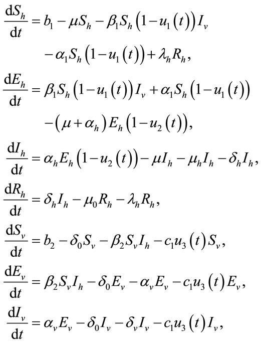
2. Basic Mathematical Model
Basic epidemic models allow for variations in the different stages(classes) of the infection. Several researcher developed different mathematical models to identifying the stages which depends on the dynamics of the disease and the composition of the population. In these mathematical models an individual can be in any one of the stages of infection. Susceptible (S), the individual is able to contract the infection; exposed (E), the individual has contracted the disease but is not yet infectious or symptomatic; infectious (I), the individual is contagious and may or may not be showing symptoms; and removed (R), an individual can be removed from the population by recovering with immunity, being quarantined or by death. In this work, we present the basic model proposed by [20], consisting a non-linear system of seven differential equations. We consider a given human population which we divide into four categories: susceptible, exposed, infected and recovered classes.
For each category, we assume the population changes over time. Thus, we write the number of humans in each category  susceptible,
  exposed,
  infected and
  recovered human as functions of time t. The total human population is denoted by
  with
with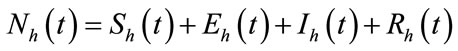 . Similarly, we write the number of vector in each category:
  susceptible,
  exposed, and
  infected vector, respectively as functions of time t. The total vector class is denoted by Nv(t) with
 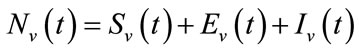 . The complete system of non-linear differential equation is given by:
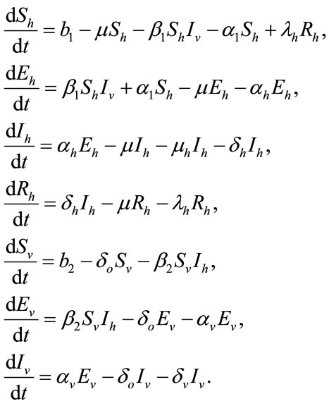 (1)
(1)
With initials conditions
 (2)
(2)
The parameters involved in the basic model are as under:
 is the recruitment rate of human population,
 is the transmission coefficient,
 is the transmission coefficient,
 is the Transmission coefficient,
 is the natural mortality rate of human,
 is the death rate of infected human,
 is the recruitment rate of vector,
 is the natural mortality rate of vector,
 is the death rate of infected vector,
 is the rate at which exposed vector move to exposed class,
 is the rate at which exposed human move to exposed class.
3. The Control Problem
Optimal control is one of the techniques to minimize (maximize) the infection in the human class of individuals. Several articles have been published on different population models by applying the optimal control techniques to reduce the infection at the human population using different control variables [17,19]. In this section, we present an optimal control technique by using multiple control variables to reduce the spread of leptospirosis infection in a community. Our educational/vaccination campaign consisting of the following control variables:
 : represents (cover all cuts, water dry, full-cover boots, shoes and long sleeve shirts when handling animals),
 : represents (wash hands thoroughly on a regular basis and shower after work),
 : represents (clean up both work place and home).
Our control strategies by using the above three control variables can be easily implemented to eradicate the spread of this disease in the community.
The control set for the control variables is defined as,
 (3)
(3)
The above control variables in the system (1) are adjusted in the following form
 (4)
(4)
with the initials conditions given in (2).
Here  represents the constant at which the rate of vector decreases at time t. The factor
  and
and , are used to reduce the force of infections.
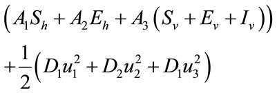
Our aim is to decrease the number of susceptible, exposed human and total vector population and increase the recovered human population. In order to do this, we define the objective functional is given by
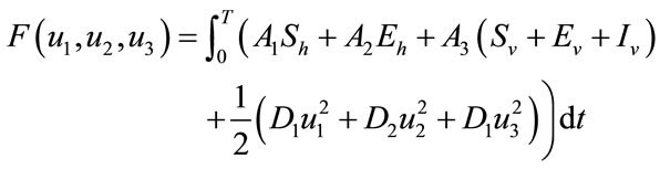 . (5)
. (5)
The objective functional includes the susceptible individuals, exposed individuals, and the class of vector population. The constants  and
and  for
for 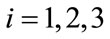 are weight/balance factors to keep the balanced of individuals in the objective functional. The Lagrange for the control problem (4) is given by
 . (6)
. (6)
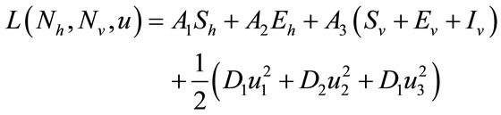
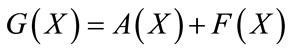
To do this, we define the Hamiltonian H for the control problem as follows:
 (7)
(7)
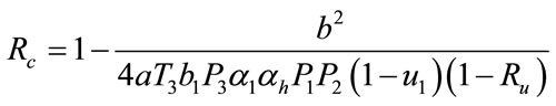
4. Reproductive Number Ro and Ru
In order to understand the dynamical behavior, we find the threshold quantity, also known as the basic reproductive number. This number is obtained by setting the right hand side of all equations equal to zero of the system (1) without control and the system (4) with control and do some rearrange to get the following two basic reproductive numbers. We obtain two reproductive numbers  and
and  form the above two systems without and with optimal control, respectively. The threshold quantity denoted by
  for the system (1) without optimal control variable is given by,
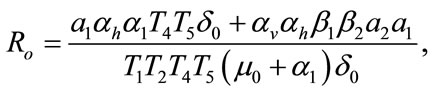
where,
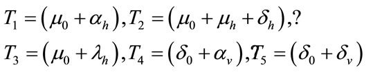
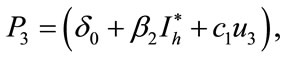
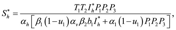
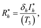
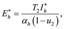
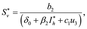
The threshold quantity  for control problem in the control system (4) is given by
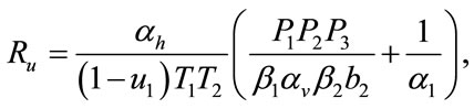
where,

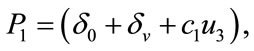

 ,
,  ,
,  and
and  are defined above for both threshold quantity
  and
and .
.
5. Endemic Equilibria and Backward Bifurcation
In this section, we find the endemic equilibria of the control system (4) and check that the backward bifurcation of the optimal control problem exists or not. For the endemic equilibria we set left hand side of the control system (4) equal to zero, to obtain
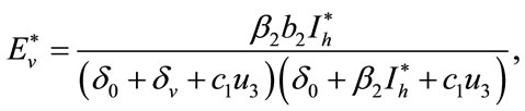
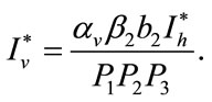
Here 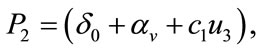
 ,
,
 ,
,  ,
, .
.
In order to find the backward bifurcation, we put the above endemic equilibria in the first equation of the system (4), with setting left hand side equal to zero to get
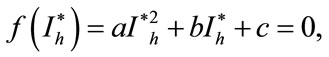
where,

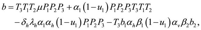
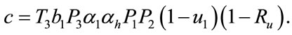
Here the coefficient a is positive always and c depends upon the value of , if the value of
 , then c is positive, otherwise negative. The positive solution of the above equation depends upon the value of b and c. For the value of
 , the above equation leads to two different roots one positive and negative. If we substitute
 , then the equation has no positive solution. This is possible if and only if b < 0. For b < 0 and
 , the equilibria depends upon
  then there exists an open interval having two positive roots that is
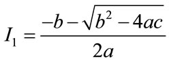 and
and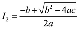 .
.
For  either
  or
or , then the above have no positive solution. For backward bifurcation, we set
 ,
,  and solving for the critical value of
 , which is given by
The numerical simulation of the backward bifurcation is obtained by using MATLAB. First we find the numerical results represented in Figures 1-3 for control variable  respectively. Figure 4 shows the numerical result without control system and Figure 5 shows the numerical result of the system with control for all the three control variables.
6. Existence of Control Problem
In this section, we show the existence of the control system (4). Let  and
and  be the state variables with control variables
 and
and . We can write the system (4) in the following form:
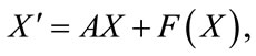 (8)
(8)
where
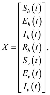
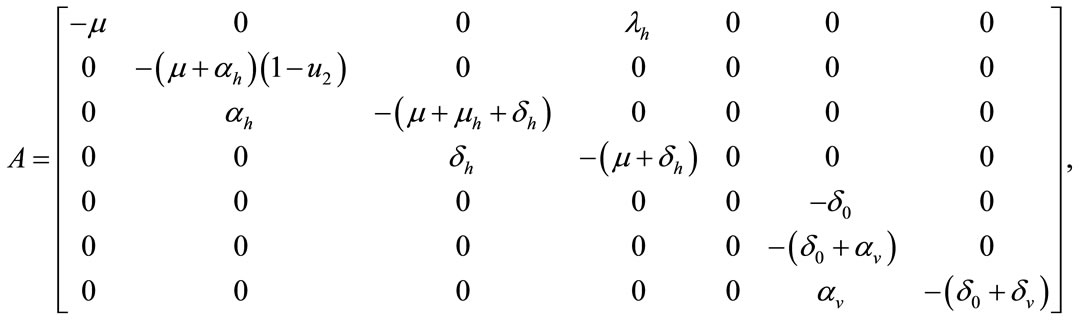
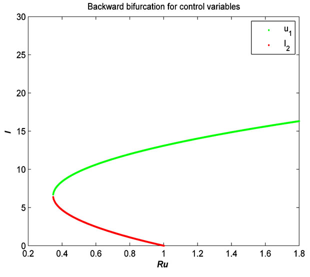
Figure 1. The plot represents the backward bifurcation for control variable u1.
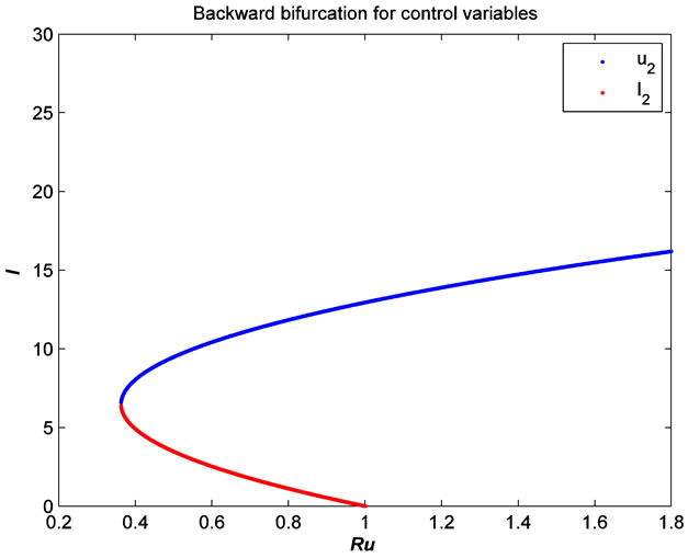
Figure 2. The plot represents the backward bifurcation for the control variable u2.
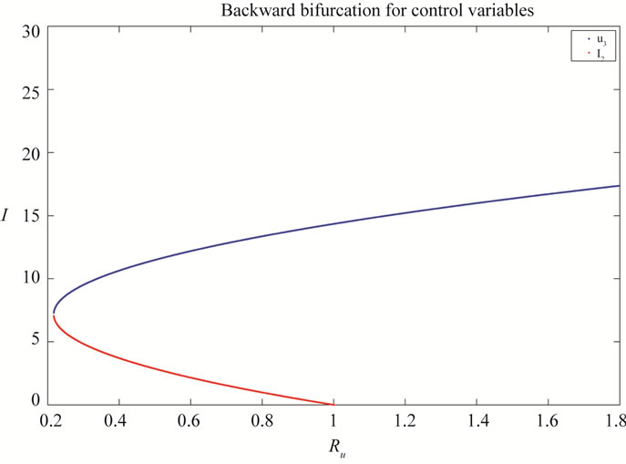
Figure 3. The plot represents the backward bifurcation for control u3.
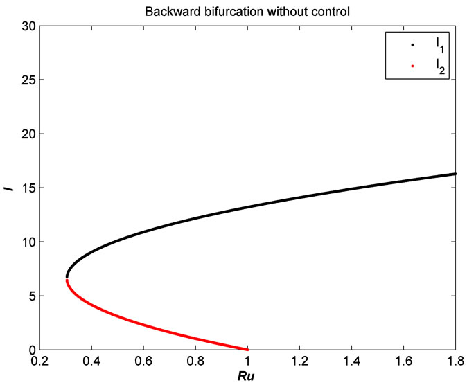
Figure 4. The plot represents the backward bifurcation without control variables.
Figure 5. The plot represents the backward bifurcation with control variables u1, u2, u3.
where  denotes the derivative with respect to time t. The system (8) is a non-linear system with bounded coefficients. We set
 , (9)
, (9)
The second term on the right hand side of (9) satisfies
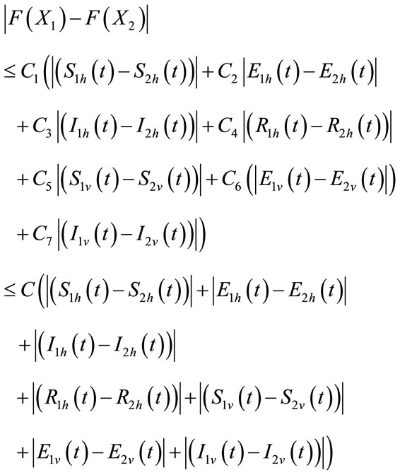
where the positive constant
 is independent of the state variables. Also we have
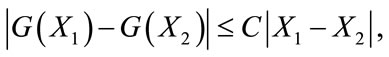
where 
So, it follows that the function G is uniformly Lipschitz continuous. From the definition of control variables and non-negative initial conditions we can see that a solution of the system (8) exists see [21]. For the existence of our control problem, we revisit the optimal control problem presented in (4) with initial conditions (2) to state and prove the following theorem.
Theorem 5.1: There exists an optimal control
 such that
 subject to the control system (4) with the initial conditions (2).
Proof: For the proof of this result, we use the same result presented in [22]. Since the control and the state variable are nonnegative. Our goal is to minimize the objective functional in the optimal control problem, the necessary convexity of the objective functional in  are satisfied. The set of control variables
  is also convex and closed by the definition. The optimal system is bounded which determines the compactness needed for the existence of optimal control. The integrand in the objective functional (5) is given by
is convex in the control set U. Also we can easily see that, there exists a constant  and positive numbers
  and
and  such that
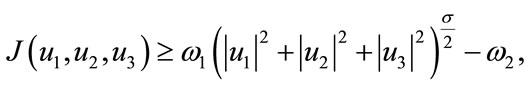
which shows the existence of an optimal control problem. 
To find the optimal solution to the control problem (4), we using the necessary conditions presented in [23,24] are given by
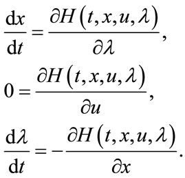 (10)
(10)
Now we apply the necessary conditions to Hamiltonian (7), for our optimal solution.
Theorem 5.2: Suppose 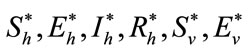 and
and  be the optimal state solutions with associated optimal control variables
 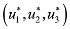 for the optimal control problem (4), with the initial conditions (2). Then there exists adjoint variables
 , for
, for  satisfying
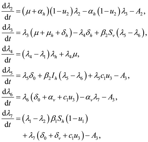 (11)
(11)
with transversality conditions (or boundary conditions)
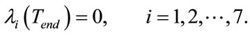 (12)
(12)
Furthermore, optimal controls  and
and  are given by
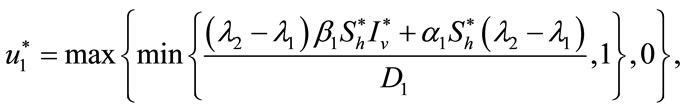 (13)
(13)
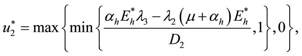 (14)
(14)
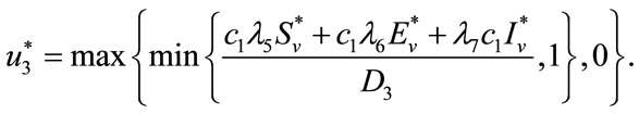 (15)
(15)
Proof: To prove the above result, i.e. the adjoint equation and the transversallity conditions, we use the Hamiltonian (7). The adjoint system was obtained by Pontryagin’s Maximum Principle [23,24].
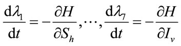 , (16)
with 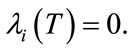 To obtained the required characterization of the optimal control given by (13) to (15), solving equations,
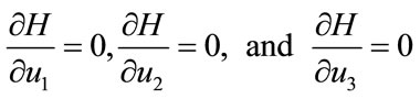 (17)
(17)
in the interior of the control set and by the control space U, we derive Equations (13) to (15).
6. Numerical Results
In this section, we present numerical simulations of the system (1) and the control system (4). We use forward Runge-Kutta order four schemes to solve both the system (1) and the control system (4). For the numerical solution of the adjoint system (11), we use backward Runge-Kutta order four schemes because of the transversality conditions or boundary conditions (12). For numerical simulation we consider parameters value presented in Table 1 using the MATLAB. Throughout this simulation we use the bold line for the system without control and the dashes line represents the control system.
Figure 6 shows the population of both the system of control and without control. The number of susceptible individuals increases in the control system than that of the system without control.
In Figure 7 the plot shows the population of exposed human in both systems with and without control. The bold line shows the population of exposed individuals in the system of without control and the dashes line shows the population of exposed individuals in the system of with control.
Figure 8 shows the population of infected individuals in both the system with and without control.
Figure 9 represents the population of susceptible vector in both the system of with and without control.
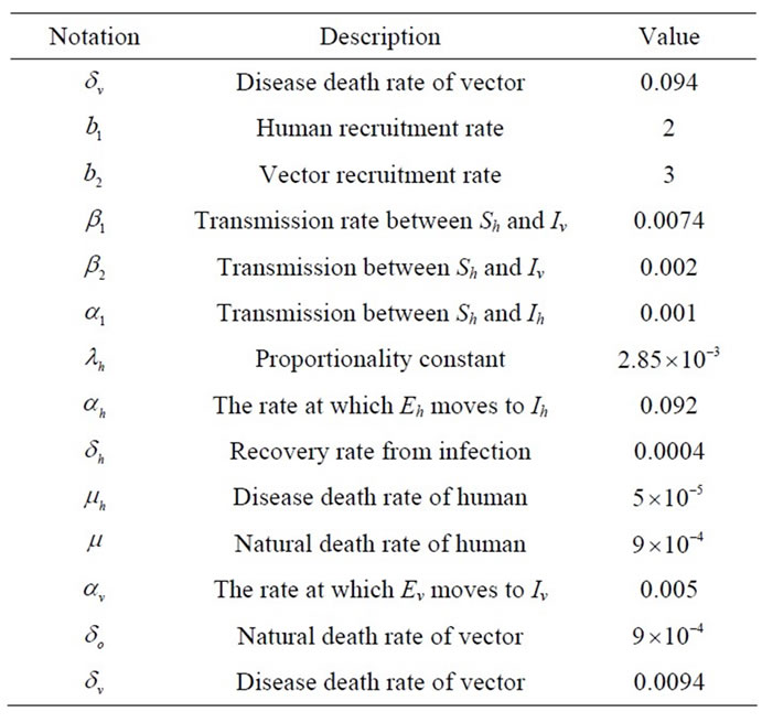
Table 1. Parameters values in the numerical simulation.
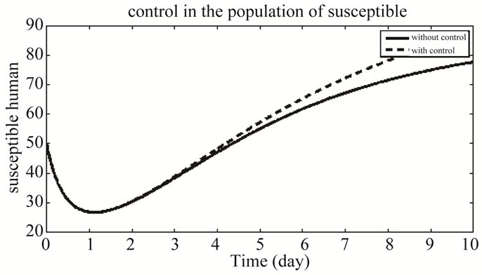
Figure 6. The plot represents the population of susceptible individuals.
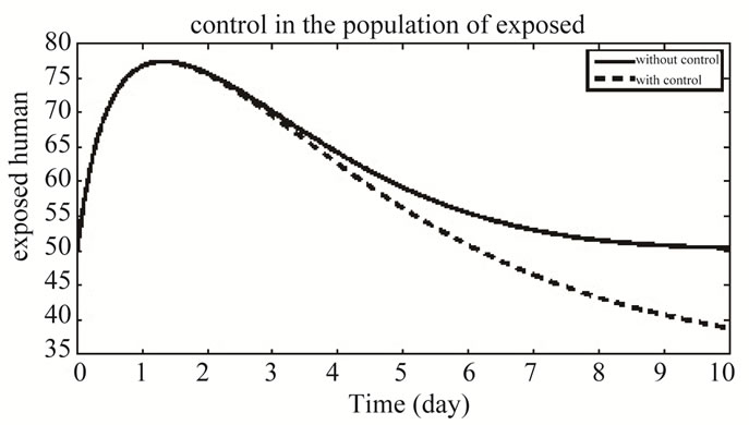
Figure 7. The plot represents the population of exposed individuals.
Figure 8. The plot represents the population of infected individuals.
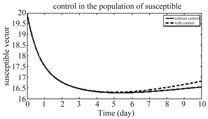
Figure 9. The plot represents the population of susceptible vector.
Figure 10 shows the population of exposed vector in both the system of with and without control system.
Figure 11 shows the population of infected vector in both the system of with and without control. Our numerical results show that the number of susceptible, exposed human and total vector population decrease and the number recovered human population increase which is the goal of this paper.
7. Conclusion
In this paper, we introduced optimal control campaign to
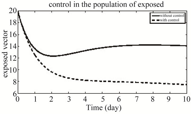
Figure 10. The plot represents the population of exposed vector.
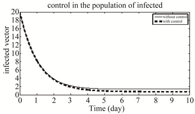
Figure 11. The plot represents the population of infected vector.
the model to maximize the population of recovered human and minimize the population of susceptible and infected human and total vector population using three control variables. First, we developed a mathematical model and then formulated the optimal control problem. We also investigated the endemic equilibria for both systems with and without control and presented their existence. We also found two basic reproductive numbers including the control variables. For certain values of these basic reproductive numbers some one can find that the disease spread in a community or not. We solved both system numerically and shown our work objective graphically.
8. Acknowledgements
The authors are very thankful to the anonymous referees for their valuables comments to improve the quality of this paper. The work of Dr. M. Ikhlaq Chohan was partially supported by the Business and Accounting Department Al Buraimi University College Al Buraimi, Oman.
REFERENCES
- R. U. Palanippan, S. Ramanujam and Y.-F. Chang, “Leptospirosis: Pathogenesis, Immunity, and Diagnosis,” Current Opinion in Infectious Diseases, Vol. 20, No. 3, 2007, pp. 284-292. doi:10.1097/QCO.0b013e32814a5729
- R. Inada and Y. Ido, “The Etiology Mode of Infection and Specific Therapy of Weil’s Disease,” Journal of Experimental Medicine, Vol. 23, No. 3, 1916, pp. 377-402. doi:10.1084/jem.23.3.377
- R. C. Abdulkader, A. C. Seguro, P. S. Malheiro, et al., “Peculiar Electrolytic and Hormonal Abnormalities in Acute Renal Failure Due to Leptospirosis,” The American Journal of Tropical Medicine and Hygiene, Vol. 54, No. 1, 1996, pp. 1-6.
- V. M. Arean, G. Sarasin and J. H. Green, “The Pathogenesis of Leptospirosis: Toxin Production by Leptospira Icterohaemorrhagiae,” American Journal of Veterinary Research, Vol. 28, 1964, pp. 836-843.
- V. M. Arean, “Studies on the Pathogenesis of Leptospirosis. II. A Clinicopathologic Evaluation of Hepatic and Renal Function in Experimental Leptospiral Infections,” Laboratory Investigation, Vol. 11, 1962, pp. 273-288.
- S. Barkay and H. Garzozi, “Leptospirosis and Uveitis,” Anmnals of Ophthalmology, Vol. 16, No. 2, 1984, pp. 164-168.
- S. Faine, “Guideline for Control of Leptospirosis,” World Health Organization, Geneva, 1982, p. 129.
- N. Chitnis, T. Smith and R. Steketee, “A Mathematical Model for the Dynamics of Malaria in Mosquitoes Feeding on a Heterogeneous Host Population,” Journal of Biological Dynamics, Vol. 2, No. 3, 2008, pp. 259-285. doi:10.1080/17513750701769857
- M. Derouich and A. Boutayeb, “Dengue Fever: Mathematical Modelling and Computer Simulations,” Applied Mathematics and Computation, Vol. 177, No. 2, 2006, pp. 528-544. doi:10.1016/j.amc.2005.11.031
- L. Esteva and C. Vergas, “A Model for Dengue Disease with Variable Human Populations,” Journal of Mathematical Biology, Vol. 38, No. 3, 1999, pp. 220-240. doi:10.1007/s002850050147
- P. Pongsuumpun, T. Miami and R. Kongnuy, “Age Structural Transmission Model for Leptospirosis,” The 3rd International Symposium on Biomedical Engineering, Bangkok, 10-11 November 2008, pp. 411-416.
- G. Zaman, M. A. Khan, S. Islam, M. I. Chohan and I. H. Jung, “Modeling Dynamical Interactions between Leptospirosis Infected Vector and Human Population,” Applied Mathematical Sciences, Vol. 6, No. 26, 2012, pp. 1287- 1302.
- W. Triampo, D. Baowan, I. M. Tang, N. Nuttavut, J. Wong-Ekkabut and G. Doungchawee, “A Simple Deterministic Model for the Spread of Leptospirosis in Thailand,” International Journal of Biological and Life Sciences, Vol. 2, No. 1, 2006, pp. 22-26.
- G. Zaman, “Dynamical Behavior of Leptospirosis Disease and Role of Optimal Control Theory,” International Journal of Mathematics and Computation, Vol. 7, No. J10, 2010, pp. 80-92.
- M. N. Ashrafi and A. B. Gumel, “Mathematical Analysis of the Role of Repeated Exposure on Malaria Transmission Dynamics,” Differential Equations and Dynamical Systems, Vol. 16, No. 3, 2008, pp. 251-287. doi:10.1007/s12591-008-0015-1
- A. A. Lashari and G. Zaman, “Optimal Control of a Vector Borne Disease with Horizontal Transmission,” Nonlinear Analysis: Real World Applications, Vol. 13, No. 1, 2012, pp. 203-212. doi:10.1016/j.nonrwa.2011.07.026
- S. Lenhart and J. T. Workman, “Optimal Control Applied to Biological Models,” Champion and Hall/CRC, London, 2007.
- G. Zaman, Y. H. Kang and I. H. Jung, “Optimal Treatment of an SIR Epedemic Model with Time Delay,” Biosystems, Vol. 98, No. 1, 2009, pp. 43-50. doi:10.1016/j.biosystems.2009.05.006
- G. Zaman, M. A. Khan, et al., “Mathematical Formulation and Dynamical Interaction of Leptospirosis Disease,” Submitted 2012.
- O. Sharomi, C. N. Podder, A. B. Gumel, E. H. Elbasha and J. Watmough, “Role of Incidence Function in VaccineInduced Backward Bifurcation in Some HIV Models,” Mathematical Biosciences, Vol. 210, No. 2, 2007, pp. 436-463. doi:10.1016/j.mbs.2007.05.012
- K. W. Blayneh, Y. Cao and H. D. Kwon, “Optimal Control of Vector-Born Disease: Treatment and Prevention,” Discrete and Continuous Dynamical Systems Series B, Vol. 11, No. 3, 2009, pp. 587-611.
- G. Birkhoff and G.-C. Rota, “Ordinary Differential Equations,” 4th Edition, John Wiley and Sons, New York, 1989.
- D. L. Lukes, “Differential Equations: Classical to Controlled,” Academic Press, New York, 1982.
- M. I. Kamien and N. L. Schwartz, “Dynamics Optimization: The Calculus of Variations and Optimal Control in Economics and Management,” 2nd Edition, Elsevier Science, Amsterdam, 1991.