Modern Economy
Vol.07 No.11(2016), Article ID:71354,28 pages
10.4236/me.2016.711124
Dynamic Structure of the Global Financial System of Systems
Khaldoun Khashanah, Yue Li
Financial Engineering Program, Stevens Institute of Technology, Hoboken, NJ, USA

Copyright © 2016 by authors and Scientific Research Publishing Inc.
This work is licensed under the Creative Commons Attribution International License (CC BY 4.0).
http://creativecommons.org/licenses/by/4.0/


Received: September 6, 2016; Accepted: October 17, 2016; Published: October 20, 2016
ABSTRACT
Purpose: This paper empirically investigates the structural evolution of global financial systems from the system of systems (SoS) view for eleven countries. The financial SoS consists of eleven countries each of which has its own financial system with relative autonomy. The paper aims to provide a prototype of the structural dynamics of the global financial SoS for the eleven financial entities during different phases of the financial markets. Methodology/Approach: The graph-theoretic approach of minimum spanning trees (MST) is applied on two levels to construct the component level of a subsystem within each country and the systemic level of global financial SoS. An SoS can be viewed as a network of networks (NoN) of financial transactions. The statistical approach of principal components analysis (PCA) is also applied to the systemic level of financial SoS among geographic countries to find the driving factor of variance. Originality/Value: This study provides an empirical quantitative measure of systemic risk and applies it to the global SoS to describe the interconnections and linkages. This paper examines the transmission of risks among the components. The structural dynamics of the SoS is expected to be a function of economic cycles including episodes of economic expansion and contraction. Findings: The average distance of component level MST is found to be lower during an economic contraction and higher during an economic expansion. The systemic level MST of global SoS can successfully reflect the geographic as well as the economic relationship between countries. The model verifies the intuition on natural clusters of Germany-France- Italy and the USA-Canada-UK as implied by the tight economic interconnections in each cluster. The result from PCA shows the USA, UK, and Australia experienced a counter movement compared to other European countries during the Euro debt crisis. The Japan financial system contraction and expansion can be explained by other countries indicating that it does not appear to be the driving factor of global SoS over the period of the data sample.
Keywords:
Principal Components Analysis (PCA), Minimum Spanning Tree (MST), Financial Systems, System of Systems (SoS), Systemic Risk

1. Introduction
The recent subprime mortgage crisis in 2008 exposed the weaknesses of the financial system both in the U.S. and globally. The U.S. regulatory system was not equipped with the financial early warning system necessary to monitor financial institutions projecting excessive systemic risk to the SoS. Kaufman [1] implies that the financial systemic risk is the probability of the collapse of the entire financial system, not just in any individual entity, group or component of such financial system. The collapse of the entire system results from the contagion effect of the shock of a single entity or a sector. Accordingly, the reason for exploring the system of systems (SoS) in financial markets is to measure the degree of relationship of its components and the transmission of risk. The systemic risk in global financial systems and economies has a critical influence on understanding the interdependence of the entire financial SoS. Evans and Hnatkovska [2] investigated how international financial integration affects the behavior of international capital flows and asset prices. They declared that international financial integration capital flows are large and volatile at the beginning stage. They also demonstrated that global risk factors have become more important in determining excess equity returns. There have been many studies on systemic risk after the crisis of 2008; a summary of approaches was given by Flood and Lo [3] . Many papers emphasize the role of the banking system [4] [5] [6] while the empirical approach emphasizes markets and the banking system. The idea comes from relating systemic risk to available information to market participants and adopting a form of efficient market hypothesis. In sufficiently transparent markets, financial and economic indicators should reflect available information including the accumulation of risks in one sector or domain of the financial system. The banking system, albeit most important in a financial system, is only one component in the SoS configuration. It moves other components such as the equities markets, housing markets, bond markets, but simultaneously the banking system is moved by changes in any of those markets. Therefore, it is important to explore the financial systems from the perspective of SoS and examine, as a whole, the relative movements of the components.
Furthermore, the financial system can be abstracted as a network problem and can be simplified as a tree structure, which is a connected undirected network without cycles. The financial SoS is an example of a network of networks or NoN, wherein each country (component) represents a network with sufficient autonomy and the collection of those country networks makes up the global NoN with regulations governing cross- boundary cash flows and risk flows. The minimum Spanning Tree (MST) algorithm has been applied to clustering behaviors of the financial system within a single financial security [7] , particularly in the U.S. financial system via stock market [8] [9] [10] or in the global financial system via FX market [11] [12] . In addition, a number of studies explore the structural evolution with dynamic MST analysis and investigate the dynamics of relationships between currencies and gold via MST analysis. The paper by McDonald shows the dynamics of currencies relationship in the global foreign exchange market and represents the countries’ geographical ties. The study [13] also confirmed that the robustness of the results from the MST method applied to the FX data. The studies [14] [15] [16] [17] point out the results that the correlation based on financial networks is an efficient method to retrieve economic information from the correlation matrix.
We conducted our research by extending the paper “Dynamic structure of the U.S. financial systems” by Khashanah & Miao [18] and empirically investigated the structural evolution of the financial system from the U.S. system to the global SoS. In the previous research, Khashanah & Miao described a simplified U.S. financial system composed of the S & P 500 index (SPX), three-month government T-bill, the U.S. dollar index (USDX), the volatility index (VIX), gold and oil. By implementing MST method introduced by Gower and Ross [19] , the results of the empirical study shows that the diameter of U.S. financial system network contracts during an economic recession and expands in an economic expansion. Moreover, the results of the principal component analysis (PCA) show the three-month T-bill was a dominant factor during the economic recession, and the VIX was the dominant factor during the economic expansion. We have implemented the idea of a simplified financial system with adding credit default swap (CDS) as an additional component and further extended the dataset to eleven countries. In this paper, we model the global SoS as in [Figure 1], which depicts the concept of an SoS as an NoN. Each node in the NoN represents a country and each country has its network of financial agents. It is observed that the basic functions of a financial system exist in all countries with variable degrees of relevance and maturity. All advanced and advancing countries are expected to have a banking system, equity market, bond market, real estates market, futures market, and a commodities and foreign exchange markets. Not all advancing countries have strongly active options market and certainly not in developing countries. Those dominant and common components of a financial system create a common architecture across different countries and that is captured in Figure 1. The volatility component is essential for representing options markets technically but, more importantly, it reflects the level of fear in markets and it is most informative in the case of the VIX. In all financial SoS architecture there are intermediaries, clearing houses, rating agencies and an infrastructure to electronically support the conduction of payments and settlements.
The methodology in this paper is designed to answer some research questions. First question is which component dominates the financial system at a given time; second what is the pattern of the co-movement in the financial markets, and how the structure of the financial system changes during the economic recession and expansion.
We apply a topological arrangement of different assets in each financial market. A node in the model represents a class of assets such as equities or bonds. Nodes of the
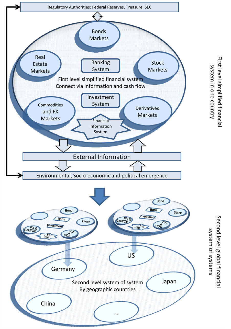
Figure 1. Prototypical financial system representing one country to global system of systems.
MST represent the component level of each country while the synthesis of responses of nodes provides intelligence at the systemic level of the SoS. The distance between two nodes is measured by utilizing correlation matrix and network similarity. The basic structure of the tree topology is robust with respect to time.
Compared to the result of the U.S. system in [Khashanah & Miao] [18] , this paper covers regions of Europe, America, and Asia, including developed countries (“G7”) and the emerging markets Brazil, Russia, India and China (BRIC). We describe the dynamics of the average distance of MST as a systemic risk indicator in the U.S. market through the entire business cycles and provide the conclusion of how a component (subsystem) expands and contracts from prosperity to turmoil. On the systemic level of SoS, we applied a similar quantitative measure that shows how structural factors transmit and how the global systemic risk is captured. The method can provide more information to individuals, institutions, regulators, and central bankers for warning or detecting an impending crisis. It also provides insight into market behavior that is not easily observed from the correlation matrix.
The rest of this paper is organized as follows. In Section 2, we briefly review the method and findings by constructing the U.S. simplified financial market, and our enhanced extension to global financial SoS. In Section 3, we describe the dataset used for this study; preliminary analysis is provided. Section 4 provides the methodology and findings from an empirical investigation using the MST approach. Section 5 uses Principal Component Analysis (PCA) to analyze our empirical dataset, and the corresponding result is shown. Section 6 concludes with the main findings.
2. Review & Extension
2.1. Review
The previous research by Khashanah& Miao [18] focused only on the U.S. financial markets with representative indicators of S&P 500 (SPX), VIX, 3-Month Treasury Bill (3-Month T-Bill), the U.S. Dollar Index (USDX), Gold and Oil to inform on different types of the financial assets as equities, derivatives, bonds, foreign exchanges and commodities to construct a simplified financial systemic and holistic view. By using the statistical approach of PCA and the graph-theoretic approach of MST, the research investigated the dynamic structure of simplified financial system during two phrases (June 2006-November 2007 and December 2007-May 2009), before and after the recent economic recession triggered by the U.S. subprime mortgages.
The method of PCA can indicate which component is dominant or what is the leading factor during each period of time. Empirical results show that the VIX and 3-Month T-Bill are the driving factors during the period of expansion and recession respectively.
The algorithm of MST is a general-purpose algorithm mainly applied in cluster analysis to explore the structure of a system. Using MST we introduce a new systemic risk indicator for the SoS. This is done by capturing the average distance of MSTs of each component in the SoS using the same correlation metric. MST distance enables the introduction of a new systemic risk indicator, and gives a quantitative measure to describe the overall stress of the financial market.
2.2. Extension
To extend the similar result to geographical global financial SoS in addition to the scope of the U.S. financial market. A systemic level of a global SoS prototype includes the G7 countries (the U.S., the U.K., France, Germany, Italy, Japan, Canada) as well as Australia , and emerging countries with fast growth gross domestic product (GDP) (China, Brazil, Russia).
Within each country, the component level financial subsystem architecture is consistent with local equity market, currency exchange rate, government 3-month bill, credit default swap (CDS), equity market volatility, gold and crude oil. In fact, among the seven components, the crude oil and gold are shared among all countries and work as a common factor in our simplified financial SoS. By adding CDS as an additional dimension, we extend the previous work in the component level simplified system since CDS provides an indicator of risk for the bond market.
To examine the events after the financial crisis caused by the subprime mortgage debacle, as well as the European the debt crisis thereafter, we extended the data set to cover not only the period of expansion and recession but also the period of initial recovery (June 2009-May 2010), the period of turmoil by European debt crisis (May 2010-July2012), and the steady recovery thereafter until March 2015.
3. Data
3.1. Data Sets
To explore the dynamic system structure for each period, we split the data into five mutually exclusive segments. The first two phases include the periods of early expansion and subprime mortgage crisis. The first phase is up to November 2007. Due to the easy credit and high-risk lending and borrowing, the global economy enjoyed a high growth rate and leverage was very high during that phase. The second phase is marked from December 2007 till June 2009 when the recession caused by the subprime mortgage was officially announced to end, according to Federal Reserve and National Bureau of Economic Research (NBER). After that, phase 3 is when global economy experienced an initial recovery because of the government stimulation and bailout plans to save the companies which were short of liquidity; and phase 4 is when the European debt crisis was triggered because respective governments were struggling to pay out their sovereign debt. In Figure 2, we can intuitively see that the European debt crisis turmoil did not have a continuous impact and caused two major financial events in 2010 and 2011. Phase 5 signals a steady recovery of the U.S. markets but with major events like the Quantitative Easing (QE) tapering and Federal Reserve quitting QE till March 2015.
As indicated, we have also extended our data set to include the stock index, stock index volatility, currency exchange rate, 3-month government bill, one year senior CDS, gold and oil commodity price to represent the financial asset of equities, derivatives, bond, foreign exchange and commodities for global financial market. The list of assets and data details is listed in Tables 1-3.

Table 1. Underlying assets in each country.
Table 2. Geographic countries.
Table 3. Date periods.
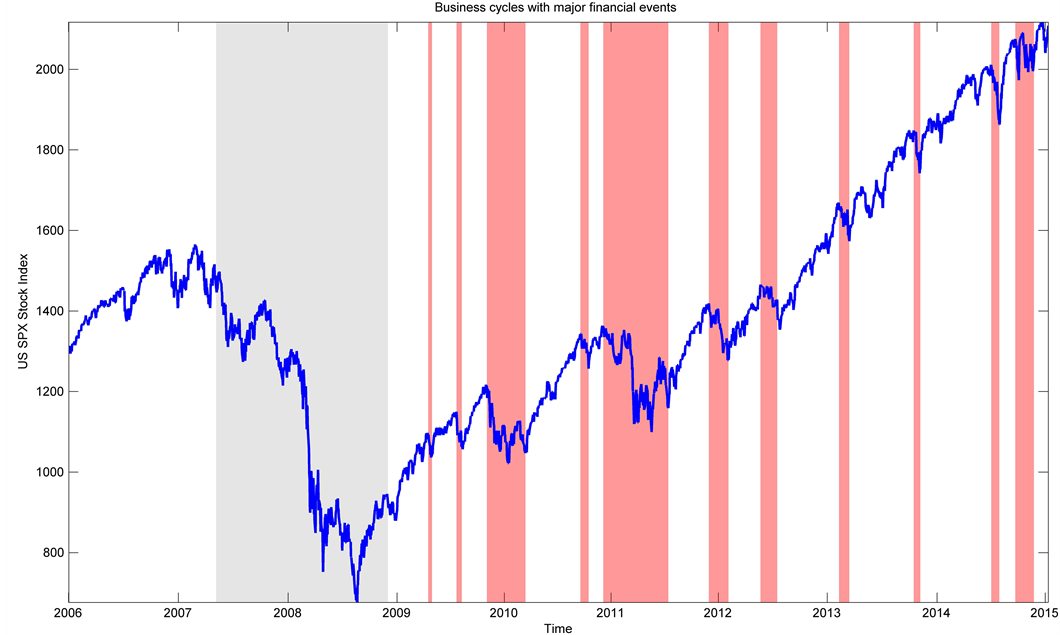
Figure 2. Business cycles with major financial events.
3.2. Raw Data Description
Figures 3-5 are the raw data plots from the seven components we use to generate subsystem signals of the global SoS. All data used are daily data in time frequency and the horizontal axis is the time from 2006 to 2015. The first group of charts in Figure 3 de- pict the bond yield from countries of the U.S., Australia, and Italy. The bond yield,
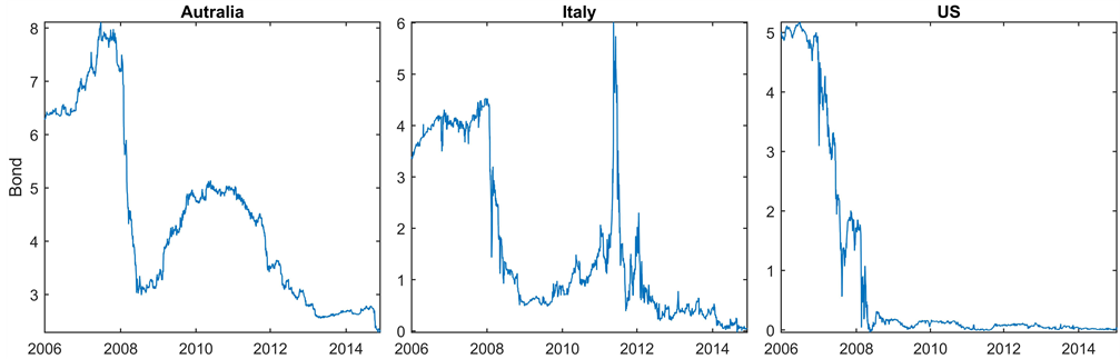
Figure 3. Bond yield comparison among Australia, Italy, and the US.
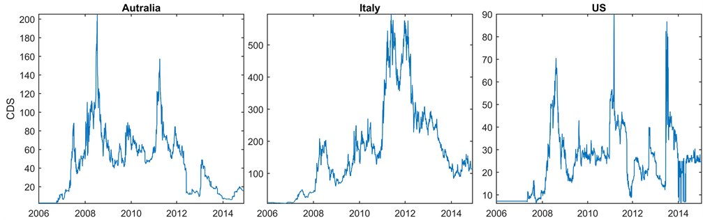
Figure 4. CDS comparison among Australia, Italy, and the US.
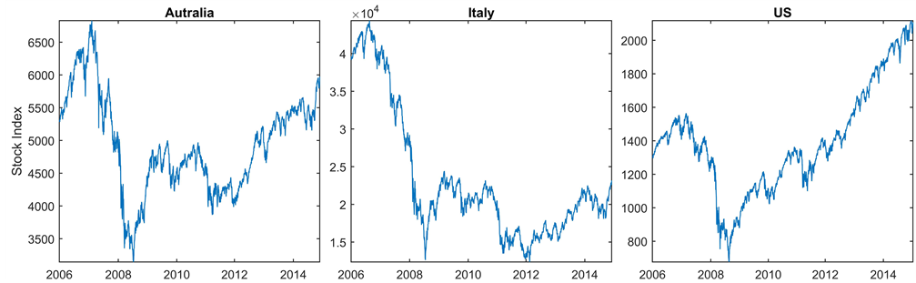
Figure 5. Stock index comparison among Australia, Italy, and the US.
which has the value of yield in percent, is one of the seven dimensions to measure the component level of the simplified financial system within each country. From the chart, we can intuitively see the bond yield trajectories have some similarities but not without major discrepancies. For Italy, it has experienced a short-term peak of bond yield because of the debt crisis; then the bond yield returned to normal after receiving support from other European countries. The European debt crisis contagion to the global economy and Australia is also reflected in component bond market signals. The bond yield in Australia increased to a local high during the period of the European debt crisis though not as significantly as in Italy’s case. For the U.S., the 3-Month T-Bill had a steady decline during the initial period then it remained near zero throughout the investigated period. When constructing the MST for the component level system, similar patterns in the dimension of the bond are factored into the similarity of the MST structure.
The second group of charts in Figure 4 concerns the CDS in each component. CDS instrument has the value of spread in basis points. For example, the CDS in Italy increased dramatically in the same period of its bond yield turmoil. Even after the bond yield reverted to its normal, the CDS market was lagging in recovery in Italy.
The third group of charts in Figure 5 represent the stock index. For the U.S., we can see the stock index represented by SPX index experienced a collapse during the subprime mortgage crisis around 2008, and then had steadily recovered afterward because of the stimulus program among other reasons. Italy’s major stock index (FTSE MIB index) also had a similar pattern to that of the U.S. during that short period. Australia stock market underwent the same pattern as well notwithstanding that stock market patterns after the crisis varies in details due to different government financial and monetary policies, including stimulus program(s).
4. Minimum Spanning Tree (MST)
4.1. MST Methodology
A spanning tree is an undirected subgraph connecting all the vertices of a graph with no cycles; A minimum spanning tree (MST)is a subgraph spanning tree with weight less than or equal to the weight of all other spanning trees. The MST may not be unique for a given graph if the edge weights are not unique. The MST as an approach in graph theory has been widely used in cluster analysis and to explore the hierarchical structure of a system. The application of the MST includes computer networks, telecommunications networks, transportation networks, water supply networks, and electrical grids. When constructing a unidirectional weighted network, we are using correlation as weights in an adjacent matrix. The weighted correlation network analysis is well known as gene co-expression network in biological networks studies of bioinformatics, which is a more comprehensive framework but what we need from it includes comparing one network with another network, and finding shared characteristics between two or more networks [20] .
The MST has been widely applied in the financial system and the exploration of the linkage of financial institutions in a network structure. Mantegna [8] used the MST method to study stocks as a network structure; Onnela et al. [10] found that the MST shrinks during financial crashes in the equity market. Not only the MST has been used to describe the equity market, but it is also applied in the FX market. McDonald et al. [11] demonstrated a geographical connection by using the MST in exchange rate. In this paper we construct the MST to provide insights into the dynamic structure of the system. Coelho et al. [7] showed that the MST tends to become more compact during the integration of international stock indices. Gilmore et al. [21] finds that the mean distances of the MST decrease over time because of stronger co-movements of these markets.
In our model design, the component level of subsystem graph G with vertices V(G) are unidirectionally connected networks. The MST of graph G is a spanning tree with the shortest overall distance. The SoS graph is denoted by G' with vertices V(G'). Thus V(G') has eleven vertices (nodes) representing eleven geographic countries. Each node has an associated time series that informs on its price or value. We can convert an MST of G to the average distance of the MST in time series or a measure of similarity between networks in time series, and then apply the MST approach to construct the systemic level structure.
The similarity between objects is often defined by a distance measure. We need to define the distance metric that will be used to generate MST and further to measure the systemic risk. As a distance measure, it has to satisfy the following properties.
Distance metric:
 (1)
(1)
The following distance function definition by Mantegna [8] is a qualified distance measure that satisfies the distance metric by using the Pearson correlation:
 (Modified correlation distance)* (2)
where  is Pearson correlation and is defined as in (3) in a local financial system within specific country:
 (3)
(3)
where <> indicates the variable mean of the investigated period, and  stands for the return in time series of i-th, j-th component in the financial subsystem.
To generate an MST, the method follows the classical Kruskal’s [22] algorithm.
4.1.1. Component Level Financial Subsystem by MST
Using time series as input data from each country, the component level financial subsystem is calculated. The return from different markets can be expressed as t-by-7 matrix as below, where t is the number of observation days in the data set.

In a unidirectionally connected network, the linkage between components V(G) is expressed by the distance of MST:
 (4)
(4)
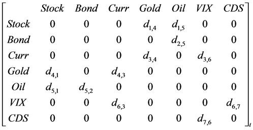
As a result from component level MST, the original network and MST can be expressed in adjacent matrix as below:
The adjacent matrix for the original unidirectional weighted correlation network:

The adjacent matrix for the generated MST:
4.1.2. Systemic Level Global Financial System of Systems
The systemic level SoS is calculated by using generated component level MST as input. There are two candidate measures to use the generated MST: average distance of MST measure and network similarity measure. We calculate the average distance of MST generated for each country as:
 (5)
(5)
Therefore, the input data for systemic level SoS can be expressed as matrix below, which is a t-by-11 matrix. The eleven dimensions are geographic countries’ time series MST data from their component level subsystems.

In Figure 6 we demonstrated that the network similarity couldbe successfully mea- sured by using average MST distance.
Next, the correlation between subsystems can be calculated by MST distance:
 (6)
(6)
Here, i, j stands for each geographic country as the SoS subsystem.
Applying MST method, the new distance of the systemic level for overall SoS is calculated as an aggregation of components correlations under the same metric as
 (7)
(7)
Alternatively, we can directly use the measure of network similarity to generate the systemic level graph from the component level MST. Here we simply adopt the Eucli-
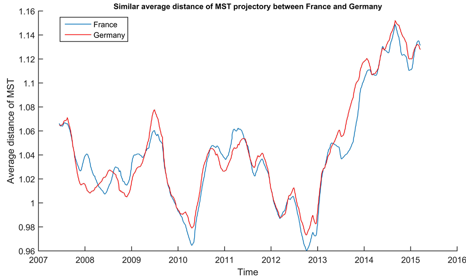
Figure 6. Similar average distance of MST trajectory between France and Germany.
dean distance as in Formulas (8) and (9). In Figure 8, we show that the two MSTs from component level financial subsystems are compared in the network similarity measure.
 (8)
(8)
 (9)
(9)
Similarly, as using average distance of MST, the correlation between subsystems can be calculated by network similarity distance:
 (10)
(10)
Alternative metric to generate systemic level MST is the same but using  in (10) as
 (11)
(11)
However, there is a drawback in applying the MST method―MST distance may not always change smoothly and may result in a sudden jump when it has accumulated a high correlation shift and trigger a structural change in the graph. To avoid the bias from a sudden shock, we need to do a moving average on the distance of MST to smooth it while still keeping the main trend. On the other hand, detecting those jumps is paramount in systemic risk investigations and is addressed with different methods. In Formula (12),  denotes the generated systemic level MST distance by using either
  or
or  measure.
Moving Average MST of SoS:
 (12)
(12)
5. Results & Findings by MST
5.1. Component Level Financial System by MST
First, we examine the component-level subsystem. Figure 6 shows the average MST distance trajectory between France and Germany, which reflects significant co-move- ment; and Figure 7 is the average MST distance between Brazil and Japan. The charts are to demonstrate the performance to measure the similarity by using average MST distance. In Figure 8, we show a comparison between the two MSTs from component level financial subsystems under the network similarity measure.
Our systemic risk coupling indicator postulated that systemic risk is inversely proportionate to the average MST distance. In other words, the lower MST distances, the higher the systemic risk. This inverse realtion between systemic risk and tight coupling can be explained in the sense of a diversication argument as well. During tight coupling all instruments produce similar patterns (highly correlated); thus, making diversivfication unattainable. The overriding systemic risk becomes the dominant signal over all other idiosyncratic component level signals of risk.
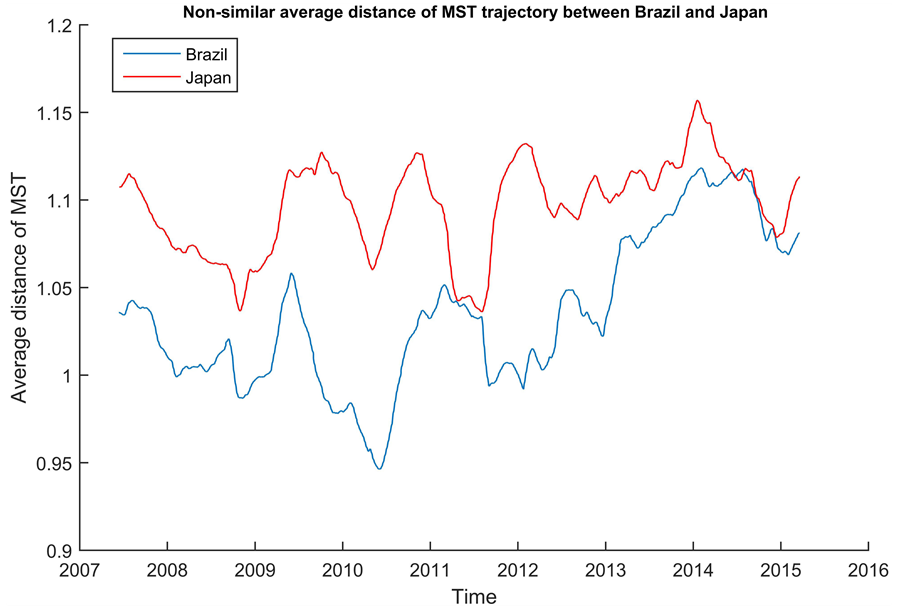
Figure 7. Dissimilarity average distance of MST trajectory between Brazil and Japan.
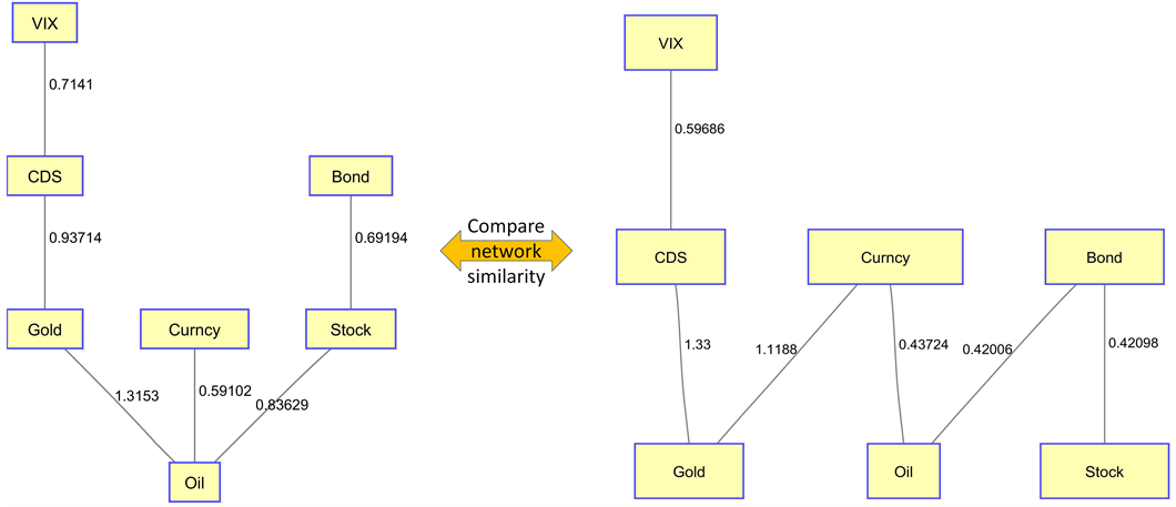
Figure 8. Comparison of Australia(left)/US(right) MSTs in network similarity measure.
In Figure 9, the average MST distance of the U.S. subsystem is compared with its stock index, which can help illustrate the time-dependent dynamic property of MST. As we can see, the average distance of the MST is at its minimum value when the stock market crashed during 2008. This result is consistent with the findings in Khashanah
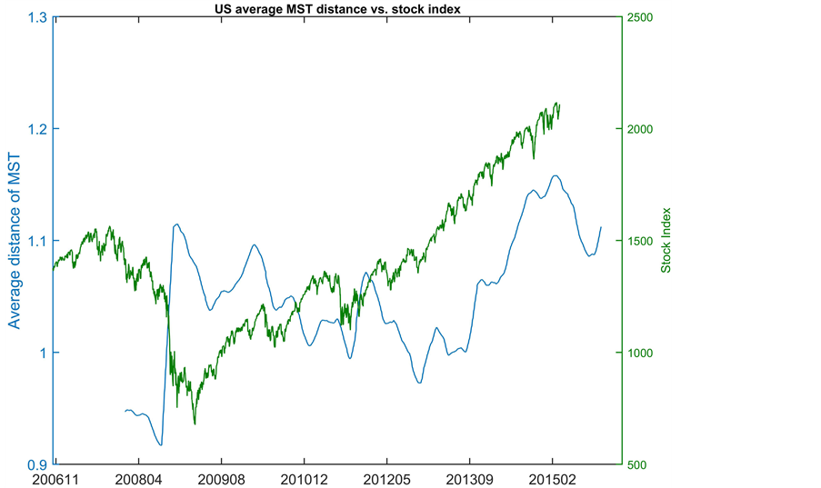
Figure 9. US average MST distance vs. stock index.
and Miao (2012)’s previous work. After that, the market started recovering, but the systemic risk within the U.S. system was not fully released during the first two rounds of quantitative easing (QE) till Sept 2012; when QE3 was announced, and the systemic risk started to reduce (average distance of the MST increasing). During the period before Sept 2012, there were two peaks in volatility which corresponded to the events of QE ending and Euro debt crisis. In the QE3 period, the stock market steadily increased with lower volatility together with reduced systemic risk. Nevertheless, the distance of MST slightly contracts after the major financial event on October 2014 but recovered a little till the end of our dataset in March 2015 (Figure 10).
5.1.1. Comparative Dynamic Structure
To further analyze the dynamics of subsystem structure, in Figure 11 and Figure 12, we show the subsystem internal structure for the U.S. financial system in different phases. They exhibit various structures during various phases. In phase 1, the oil and gold were still directly connected to each other to form a small group, as well as CDS and VIX to form another group. This phenomenon may be interpreted in terms of the nature of the financial instruments as both oil and gold represent the commodities market while both VIX and CDS reflect market fears. Stocks are closer to the commodity markets since commodities behave more like investment instruments in the U.S. In phase 2, the dynamics of MST show the structural change in the subsystem and the USD index moved to the center of the structure and worked as a bridge. Oil and gold still perform like investment instruments as they closely connect to stocks, and the overall system was connected tighter than in phase 1 as the average distance of MST was smaller.
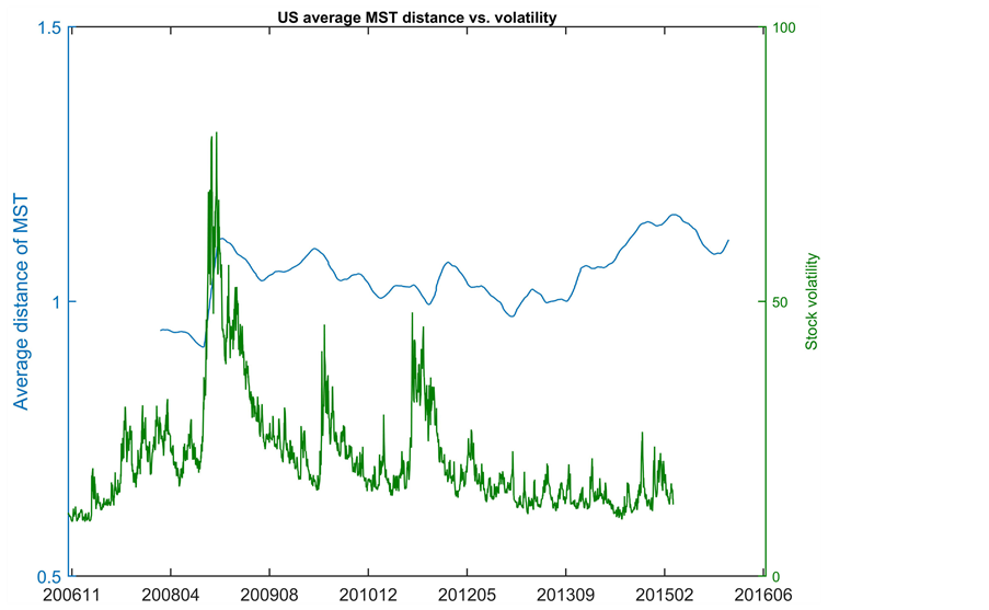
Figure 10. US average MST distance vs. volatility.
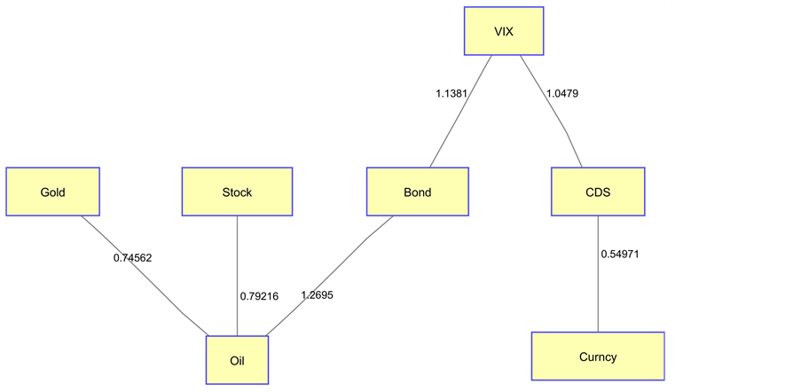
Figure 11. US financial system in phase 1.
As shown in Figure 11 and Figure 12, our MST method on the component level can generate the internal structural linkages of local simplified financial subsystem. This component level system structure can be used to compare the subsystem at a different phases so as to explore the system dynamically. Furthermore, comparing system structure with other subsystems can also be revealing to the contribution of the risk of the subsystem to the overall SoS risk. Australia’s financial subsystem structure is shown in
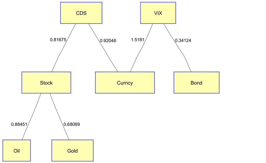
Figure 12. US financial system in phase 2.
Figure 14 while, for comparison, the U.K. financial subsystem structure is shown in Figure 15 to reveal the structural differences between the two financial entities.
5.1.2. Comparative Structure of Countries
In Figure 14 and Figure 15, both subsystem structures reflect system dynamics for the phase of original expansion. Figure 13 is the full graph before applying the MST. When applying the MST, we may lose some information but can expose the network basic structure. In Figure 14, we can see that the crude oil is the center of the network for Australia, where oil represents commodities in our simplified financial system. This is consistent with our expectation for Australia since Australia is mainly a resource- exporting country and its economy has a high correlation with commodity prices. From the same chart, it shows that the Australian dollar node has the smallest distance to the oil node. Another phenomenon that we may need to pay attention to is that both CDS and VIX are linked to the bond node. The VIX and CDS show tight co-movement because both act as fear gauges in their respective domains, which reflect the concerns and anxieties of the financial market in the future. Therefore, it makes the most sense to have both fear gauges highly correlated to each other on the systemic level.
Considering Figure 15, the system structure for the U.K. provides a different subsystem structure. Despite the oil node being still in the center of the chart, not many of the components are connected to the oil node in the U.K. system. We can unfold the chart to see that oil is simply a component in a line structure. This can be explained by the U.K.’s economy is quite different from Australian economy. For the U.K., bonds and currency are closer to the center of the system in the same plotting period.
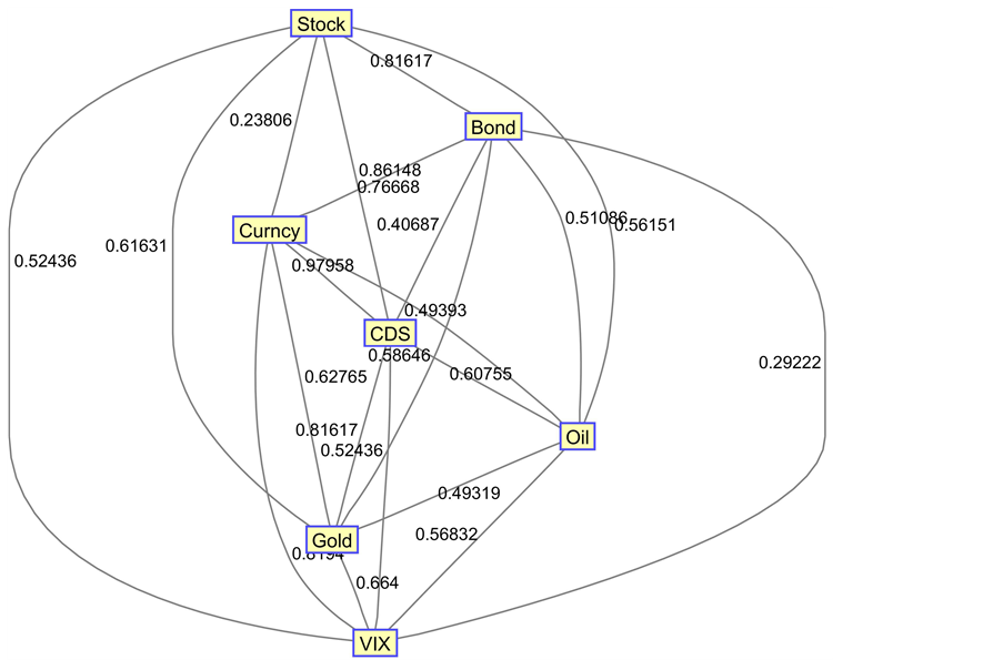
Figure 13. Australian financial system full network graph.
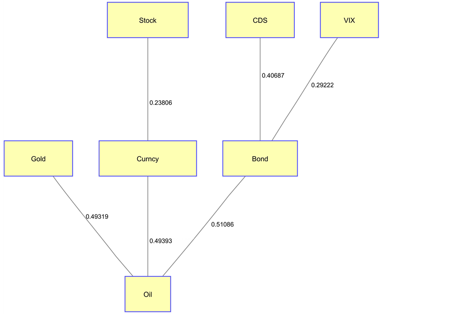
Figure 14. Australian financial system MST.
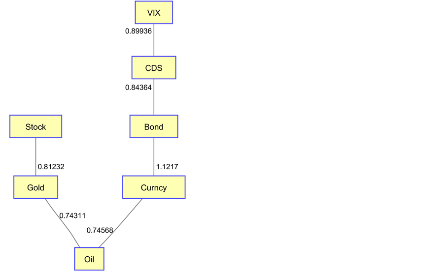
Figure 15. US avg MST distance vs. volatility.
5.2. Systemic Level SoS by Global Geographic Countries
In this section, we analyze the results from the systemic level MST, which represents simplified global financial SoS. On the systemic level, eleven geographic countries constitute a bigger global financial market. The interactions among the SoS compo- nents represent trasactions mainly through international cash flows, exchange of goods and services, imports and exports and many other financial economic activities. In our simplified model, since the interactions are transactions, they can be approximately explained by correlations among the financial markets belonging to different countries. However, each component, as a country, enjoys a certain level of autonomy that generates independent risks to the global SoS. Those component risks are either contained inside the component or, because of size, spill over to the rest of the SoS with a contagion mechanism. The condition of “size” means that the risk presents a sizable problem proportionate to the SoS capitalization. With an assumption of market efficiency, the issue of size does not appear in the approach we implement because the signals of markets are supposed to contain that assessment through pricing and valuation and, thereby, the returns must reflect the size of a given risk.
Some countries have a closer relationship with other countries due to geographic proximity or tighter economic connections like Germany, France, and Italy, which can be seen that they tend to move together in a global SoS and perhaps as a form a small network community.
Under the similarity measure used in this paper, Figure 16 shows the result from the systemic level MST of SoS. This system structure is generated by purely using financial
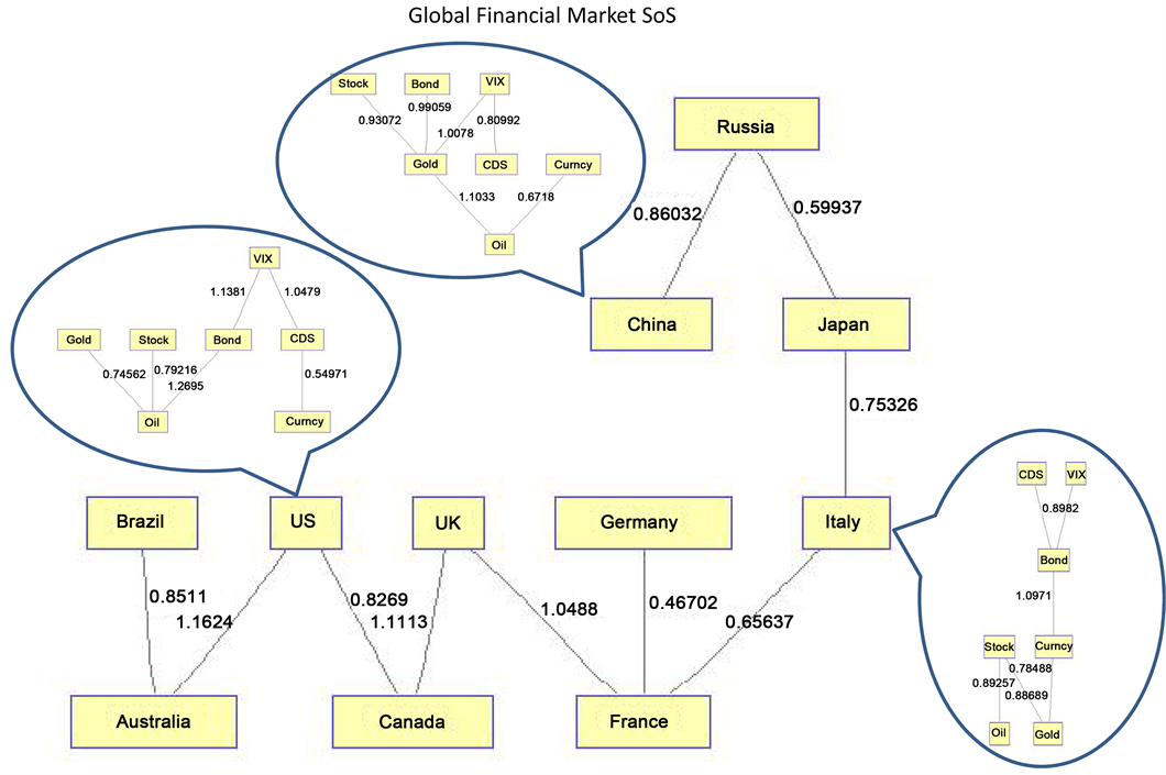
Figure 16. Global financial market system of systems.
instruments data but can indeed reflect a natural clustering reflecting geographic proximity. From Figure 16, the U.S., Canada, and the U.K. are more tightly connected to each other and form a small group within global SoS topology (this is true except for the period of European debt crisis). In addition, Germany, France and Italy form another tightly connected small group. Within each subsystem, the component level system architecture consists of seven financial instruments, and each country may have its own dynamic structure as a subsystem.
Dynamic Structure of SoS across Different Phases
By dividing the data sample period into different phases, we can get a clear picture of how the system structure evolves during the business cycle by comparing the MST structures across different phases. In Figures 17-19 the MST plotting of global financial SoS in each phase during the recession, initial recovery and European debt crisis are shown and analyzed below.
1) Recession
During the subprime crisis, lots of countries’ economy was tied with the U.S. because the U.S. was the source of the subprime crisis. The contagion effect transmitted from the U.S. to other countries. However, the result demonstrated in Figure 17 shows that
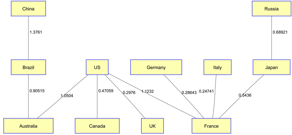
Figure 17. MST of global financial SoS during recession.
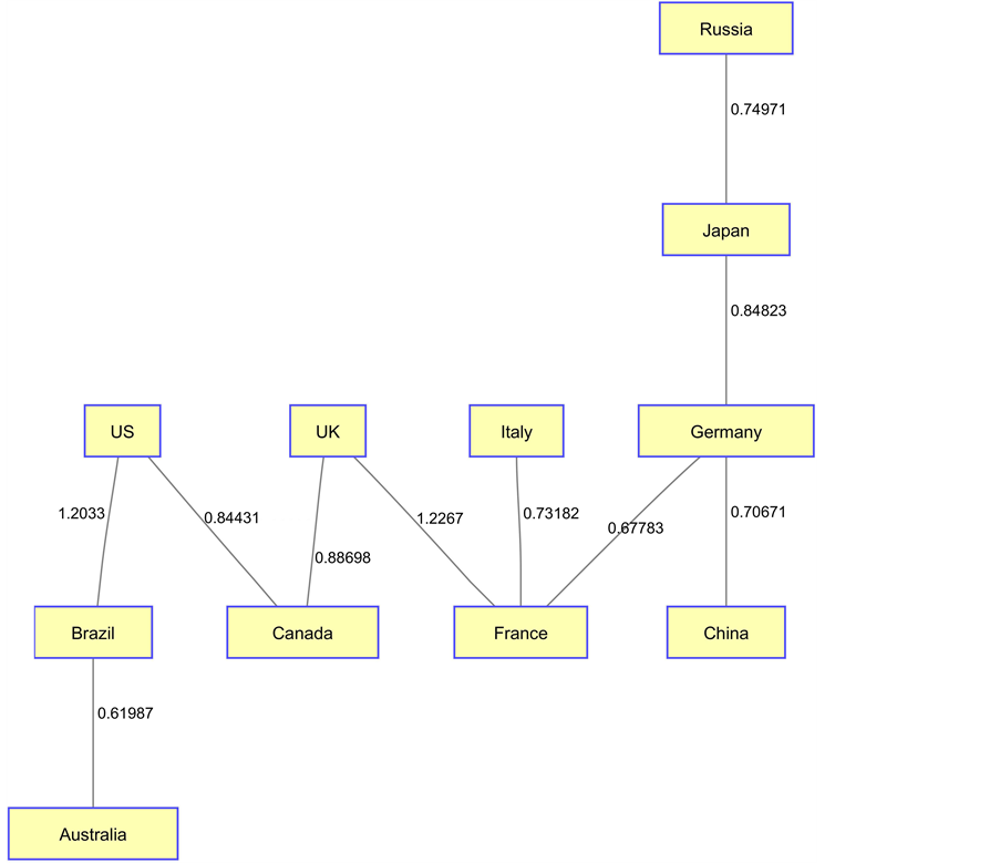
Figure 18. MST of global financial SoS during initial recovery.
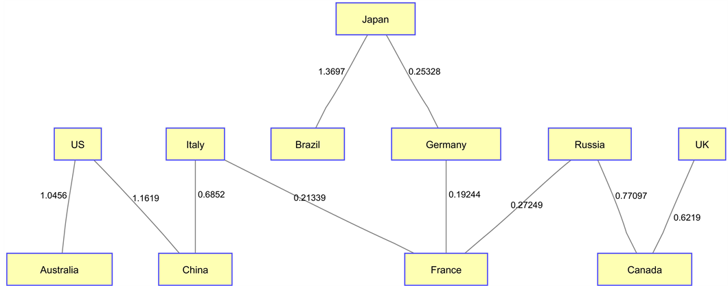
Figure 19. MST of Global financial SoS during european debt crisis.
China and Russia may be seen as the recipient of minimum impact during the crisis phase. During the recession, we can see the MST distance between the U.S. and Canada (0.47), between the U.S. and the U.K. (0.3) were much shorter than their neighborhood, and thus we observe the so-called a clique or small group phenomenon. Similarly, the distance between Germany and France (0.29), Italy and France (0.25) were also much shorter and formed another group. This can be thought of as evidence of countries with close economic relationships, and our method of SoS can successfully reflect the connections and impact of geography or other forms of proximity.
2) Recovery
In the period of initial recovery, the U.S. was still the center of the system but not tightly connected with all the other countries as in the phase of recession. China and Germany were moving closer and to the center of the SoS as main growth engines of the global economy during the initial recovery period. During this period, the U.S., the U.K., and Canada were still in the same group, as well as Italy, France and Germany. However, the MST distance had been much wider during this initial recovery period. China and Japan also had a similar distance to Germany. All this can be explained as SoS tend to be diversified while in the expansion. Also to be noticed that Brazil and Australia are connected with a very short distance indicating similarity mainly due to the observation that both economies heavily rely on resource exporting, and the commodities prices have a huge impact during the initial recovery phase.
3) European Debt Crisis
During the European debt crisis phase, the small group (clique) of the U.S.-Cana- da-the U.K. broke which we explained as the U.S. was not impacted as much as the U.K. and other European countries because of the Quantitative Easing (QE) program. Meanwhile, European countries like Germany, France, and Italy were still tightly connected to each other; and now Germany-France-Italy community had moved to the center of the system, and worked as a driving factor in the global economy.
6. Principal Component Analysis (PCA)
6.1. PCA Methodology
The PCA is a well-established method especially in reducing dimensions, which can extract feature vectors by projecting value from the old space into the rotated new space so that fewer principal dimensions in the new space can represent most of the variance in the old space.
 (13)
(13)
where C is the covariance matrix, and V is eigenvectors, with property of , and D is diagonal matrix of eigenvalues of C. Then PCA transform and PCA inverse transform (reconstruction) can be expressed as (14) (15). Here we can use a reduced dimension to separate main signal and noise.
 (14)
(14)
 (15)
(15)
Applying PCA on the systemic level SoS to the distance time series t-by-11 matrix, we decompose the covariance matrix into orthogonal principal components and corresponding loading factors.
6.2. Result from PCA
In Tables 4-6, we demonstrate the result from PCA during different phases of the business cycle. Unlike the PCA result on the component level financial subsystem within each country, it is hard to tell which country is the driving factor to the global SoS.
Table 4. PCA for period of european debit crisis.
Table 5. PCA for period of QE3.
Table 6. PCA for overall period.
During the period of European Debt Crisis, the U.K., the U.S., and Australia were having opposite loading factor to the other countries (including European countries, emerging countries, and Japan). This is seen as the counter movement on the systemic risk level. While the U.S., the U.K., and Australia were less contributing to systemic risk, European countries were experiencing an increase in systemic risk, which is an indication of diffusion of risk to through contagion to other emerging countries during that period, as well as to Japan. But due to the variance explained by first principal component (factor 1) is only about 49%, we need to combine the first two principal components together to make a comparison. For the factor 2, the sign was all positive, which indicates the directions of change in systemic risk were all the same by second principal component. The second factor can explain about 26% of the total variance.
During the phase 5 of QE3, when the U.S. experienced a steady recovery and European countries still struggled, the global SoS dictates that the systemic risk from global view were moving towards the same direction. Although it is still hard to determine which country is the driving factor of global systemic risk, we can at least say that Japan is NOT the dominant factor during this and previous phase.
In the overall period of our experiment data, due to the average loading factors value, it is not conclusive as to which country behaves as the driving factor of systemic risk to the global SoS. However, we can tell that Japan is the least dominant factor by using the PCA analysis on the systemic level of global SoS. Here, since the first principal component can only explain about 65% of total variance, we need to combine the first and the second principal components. But both factor 1 and factor 2’s value of Japan results is relatively small numbers. Here we can view as Japan’s financial system’s contraction and expansion can be explained by other countries (i.e. U.S.), but it is not the driving factor of global SoS at least in our experiment data set.
7. Conclusions
In this paper, we use a common architecture for each component country in the SoS. The architecture includes markets of relevance as indicators of accumulated systemic risk in their respective country. Instruments include CDS financial products, equities, bonds, currencies, derivatives, and commodities; we add one more dimension for data sources to reflect the fear or anxiety of the bond market. By extending the data set after the initial recovery of the subprime crisis, and covering the European debt crisis thereafter, we verified through monitoring the performance of the systemic risk measure and dynamic system structure by MST that our approach can capture the SoS accumulated systemic risk from component signals.
In the component level of the simplified financial subsystem constructed by MST, we analyze the structure difference by different countries and by different periods of time for the same country. As a systemic risk measure, the average distance of MST is lower during economic contraction since market tends to move in the same behavior and direction, while the average distance of MST is higher during economic expansion.
Furthermore, the constructed systemic level global financial SoS by eleven countries can reveal the dynamics of system structure from global economic linkages during different phases of the economic cycle. Due to a tight economic relationship or geographic location, countries can form a co-movement community in SoS. A comparison of global financial market structure for different phases has been carried out to demonstrate the driving economic entities (a single country or a small group).
The result from PCA shows the U.S., the U.K., and Australia experienced a counter movement compared to other European countries from global systemic risk perspective during the Euro debt crisis. It is hard to determine which country is the driving factor by using PCA. However, Japan’s financial system contraction and expansion can be explained using other countries co-movements. Therefore, Japan’s financial system is not driving factor of global SoS during the experiment data period.
There are also some other findings made in our study of the empirical data set. On the component level of the simplified local financial subsystem, our MST can successfully reflect the structure of the economy such as Australia may rely more on the resource exporting represented by the commodity prices. On the systemic level of global SoS, the constructed MST can successfully reflect the geographic as well as the economic relationship between countries. Germany-France-Italy community is tightly coupled similarly for the U.S.-Canada-the U.K. group. It is important to point out that while the methods of systemic risk have been successful in interpreting what happened in the financial system, the real aim is to convert this methodology and others into an early warning system for systemic risk accumulation in a SoS, which will be the subject of upcoming research.
Cite this paper
Khashanah, K. and Li, Y. (2016) Dynamic Structure of the Glo- bal Financial System of Systems. Modern Economy, 7, 1303-1330. http://dx.doi.org/10.4236/me.2016.711124
References
- 1. Kaufman, G. (2000) Banking and Currency Crises and Systemic Risk: Lessons from Recent events. Economic Perspectives, 3, 9-28.
- 2. Evans, M.D.D. and Hnatkovska, V. (2005) International Capital Flows, Returns and World Financial Integration. NBER Working Paper No. 11701, National Bureau of Economic Research, Inc., October.
- 3. Bisias, D., Flood, M., Lo, A.W. and Valavanis, S. (2012) A Survey of Systemic Risk Analytics. U.S. Department of Treasury, Office of Financial Research No. 0001.
- 4. Freixas, X., Parigi, B.M. and Rochet, J.C. (2000) Systemic Risk, Interbank Relations, and Liquidity Provision by the Central Bank. Journal of Money, Credit and Banking, 32, 611-638.
http://dx.doi.org/10.2307/2601198 - 5. Nier, E., Yang, J., Yorulmazer, T. and Alentorn, A. (2008) Network Models and Financial Stability. Working Paper 346, Bank of England.
- 6. Ladley, D. (2013) Contagion and Risk-Sharing on the Inter-Bank Market. Journal of Economic Dynamics and Control, 37, 1384-1400.
http://dx.doi.org/10.1016/j.jedc.2013.03.009 - 7. Coehlo, R., Gilmore, C. and Lucey, B.M. (2007) The Evolution of Interdependence in World Equity Markets Evidence from Minimum Spanning Trees. Physica A: Statistical Mechanics and Its Applications, 376, 455-466.
http://dx.doi.org/10.1016/j.physa.2006.10.045 - 8. Mantegna, R.N. (1999) Hierarchical Structure in Financial Markets. The European Physical Journal B-Condensed Matter and Complex Systems, 11, 193-197.
http://dx.doi.org/10.1007/s100510050929 - 9. Bonanno, G., Lillo, F. and Mantegna, R.N. (2000) High-Frequency Cross-Correlation in a Set of Stocks. Quantitative Finance, 1, 96-104.
http://dx.doi.org/10.1080/713665554 - 10. Onnela, J.-P., Chakraborti, A., Kaski, K., Kertesz, J. and Kanto, A. (2003) Dynamics of Market Correlations: Taxonomy and Portfolio Analysis. Physical Review E, 68, Article No. 056110.
http://dx.doi.org/10.1103/physreve.68.056110 - 11. McDonald, M., Suleman, O., Williams, S., Howison, S. and Johnson, N.F. (2005) Detecting a Currency’s Dominance or Dependence Using Foreign Exchange Network Trees. Physical Review E, 72, Article No. 046106.
http://dx.doi.org/10.1103/physreve.72.046106 - 12. McDonald, M., Suleman, O., Williams, S., Howison, S. and Johnson, N.F. (2008) Impact of Unexpected Events, Shocking News, and Rumors on Foreign Exchange Market Dynamics. Physical Review E, 77, Article No. 046110.
http://dx.doi.org/10.1103/physreve.77.046110 - 13. Naylora, M.J., Rose, L.C. and Moyle B.J. (2007) Topology of Foreign Exchange Markets Using Hierarchical Structure Methods. Physica A: Statistical Mechanics and its Applications, 382, 199-208.
http://dx.doi.org/10.1016/j.physa.2007.02.019 - 14. Bonanno, G., Caldarelli, G., Lillo, F., Micciche, S., Vandewalle, N. and Mantegna, R.N. (2004) Networks of Equities in Financial Markets. The European Physical Journal B, 38, 363-371.
http://dx.doi.org/10.1140/epjb/e2004-00129-6 - 15. Lehar, A. (2005) Measuring Systemic Risk: A Risk Management Approach. Journal of Banking & Finance, 29, 2577-2603.
http://dx.doi.org/10.1016/j.jbankfin.2004.09.007 - 16. Binici, M., Koksal, B. and Orman, C. (2012) Stock Return Comovement and Systemic Risk in the Turkish Banking System. MPRA Paper No. 38663, posted 8 May 2012
- 17. Patro, D.K., Qi, M. and Sun, X. (2013) A Simple Indicator of Systemic Risk. Journal of Financial Stability, 9, 105-116.
http://dx.doi.org/10.1016/j.jfs.2012.03.002 - 18. Khashanah, K. and Miao, L. (2011) Dynamic Structure of the U.S. Financial Systems. Studies in Economics and Finance, 28, 321-339.
http://dx.doi.org/10.1108/10867371111171564 - 19. Gower, J. and Ross, J. (1969) Minimum Spanning Trees and Single Linkage Cluster Analysis. Journal of Applied Statistics, 18, 54-64.
http://dx.doi.org/10.2307/2346439 - 20. Langfelder, P. and Horvath, S. (2008) WGCNA: An R Package for Weighted Correlation Network Analysis. BMC Bioinformatics, 9, 559.
http://dx.doi.org/10.1186/1471-2105-9-559 - 21. Gilmore, C.G., Lucey, B.M. and Boscia, M. (2008) An Ever-Closer Union? Examining the Evolution of Linkages of European Equity Markets via Minimum Spanning Trees. Physica A: Statistical Mechanics and Its Applications, 387, 6319-6329.
http://dx.doi.org/10.1016/j.physa.2008.07.012 - 22. Kruskal, J.B. (1956) On the Shortest Spanning Subtree of a Graph and the Traveling Salesman Problem. Proceedings of the American Mathematical Society, 7, 48-50.
http://dx.doi.org/10.1090/S0002-9939-1956-0078686-7
Appendix: Proof of Distance Metric

Normalized 
Therefore, will have .
.

Take n records of Stock i in interval as n dimensions


Submit or recommend next manuscript to SCIRP and we will provide best service for you:
Accepting pre-submission inquiries through Email, Facebook, LinkedIn, Twitter, etc.
A wide selection of journals (inclusive of 9 subjects, more than 200 journals)
Providing 24-hour high-quality service
User-friendly online submission system
Fair and swift peer-review system
Efficient typesetting and proofreading procedure
Display of the result of downloads and visits, as well as the number of cited articles
Maximum dissemination of your research work
Submit your manuscript at: http://papersubmission.scirp.org/
Or contact me@scirp.org