Journal of Environmental Protection
Vol.5 No.10(2014), Article ID:48324,9 pages
DOI:10.4236/jep.2014.510092
Research on Measurement Technology of Flue Gas Velocity Based on Optical Scintillation Induced by Fluctuation of Particulate Concentration
Zhibo Ni1, Tao Pang1, Yang Yang1, Fengzhong Dong1,2*
1Anhui Provincial Key Laboratory of Photonic Devices and Materials, Anhui Institute of Optics and Fine Mechanics, Chinese Academy of Sciences, Hefei, China
2University of Science and Technology of China, Hefei, China
Email: *fzdong@aiofm.ac.cn
Copyright © 2014 by authors and Scientific Research Publishing Inc.
This work is licensed under the Creative Commons Attribution International License (CC BY).
http://creativecommons.org/licenses/by/4.0/


Received 21 April 2014; revised 16 May 2014; accepted 8 June 2014
Abstract
Based on the theory of optical scintillation induced by fluctuation of particulate concentration, a Gas Flow Velocity Measurement System (GFVMS) is proposed to measure the gas flow velocity in stack. Verification experiments on simulation flue indicate that, for the smoothing effect of transmitting and receiving apertures, optical scintillation induced by refractive index fluctuation is very weak. When particles are added into gas flow, the standard deviation of optical scintillation increased obviously. And when the particulate number concentration exceeds 4000/m3, the GFVMS can work normally, and the variation range of measured velocities is almost the same with that of Pitot tube. Sensitivity testing results show that, GFVMS is very sensitive to velocity change. Results of outfield experiment prove that, velocities measured by GFVMS are more stable and the average velocity (7.62/s) is very close to the statistical average (7.61 m/s) of velocities measured by Pitot tube at different points along optical path.
Keywords: Optical Scintillation, Flue Gas Velocity, Particulate Concentration, Cross Correlation

1. Introduction
With the rapid development of industry, the air quality of China becomes worse and threatens human health seriously. In recent years, Chinese government has paid more attention to these problems, and a series of measures have been established and implemented to improve the air quality. To keep the effect, the control of pollution resources is of great importance. As for air pollution, particulate matters and waste gas are the main pollutants, and statistical results indicate that industrial emission is one of the major sources. Thus, monitoring the total industrial emissions of particulate matters and waste gas is crucial. During this process, the online measurement of flue gas emission velocity is indispensable.
Classical instruments for gas flow velocity measurement include Pitot tube, hot wire anemometer, and laser anemometer, et al. [1] -[3] . The measurement of Pitot tube and hot wire anemometer belongs to intrusive measurement. They can disturb flow field and lead to inaccuracy of measurement results. The advantages of laser anemometer include nonintrusive measurement, high spatial resolution and fast dynamic response. But the measurement accuracy may be affected by several factors, such as the finite measurement volume, frequency expansion, noises, etc. Based on the optical scintillation induced by refractive index fluctuation, Wang [4] proposed a new method to measure gas flow velocity. Nowadays, this method has been used in aluminum industry. Optical Flow Sensor (OFS) [5] can measure gas flow velocity with a shorter optical path, and has been designated to be the technical criterion for monitoring gas flow velocity by Environmental Protection Agency (EPA) of USA. When the temperature of flue gas is high and refractive index fluctuates obviously, optical scintillation induced by refractive index fluctuation is easy to be detected [6] . But when the fluctuation is weak, the measurement work becomes difficult. Based on optical scintillation induced by particles shifting in and out of light beam, gas flow velocity can also be measured [7] -[9] . But when the number concentration of particles is high and the diameters are small, this method is helpless [10] .
In order to develop a new instrument for gas flow velocity measurement, the relationship between optical scintillation and extinction coefficient of particles is deduced, and a Gas Flow Velocity Measurement System (GFVMS) is designed. The corresponding test experiments are carried out on simulation flue in lab and industrial stack, respectively.
2. Measurement System and Principle
The structure of GFVMS is shown in Figure 1, in
which the direction of gas flow is along y axis. The GFVMS has two parallel optical
paths in the longitudinal section of stack, and the distance between two optical
paths is . The transmitters locate
at one side of the stack, and their light sources are point sources. The detectors
locate at the opposite side of the stack, and the distances from transmitters to
detectors are both L. After collimated by transmitting lens, the probing beams propagate
to the receivers along x axis which coincide with the diameter of stack. When the
probing beams reach the receivers, light is collected by the receiving lenses.
. The transmitters locate
at one side of the stack, and their light sources are point sources. The detectors
locate at the opposite side of the stack, and the distances from transmitters to
detectors are both L. After collimated by transmitting lens, the probing beams propagate
to the receivers along x axis which coincide with the diameter of stack. When the
probing beams reach the receivers, light is collected by the receiving lenses.
To ensure the discharge velocity, blower is indispensable for industrial stack. It is the existence of blower near the entrance, gas flow entering into stack is turbulent. And it tends to be stable gradually as flowing along stack. According to the theory of turbulence, the evolution of turbulence is large eddies breaking up to small ed-
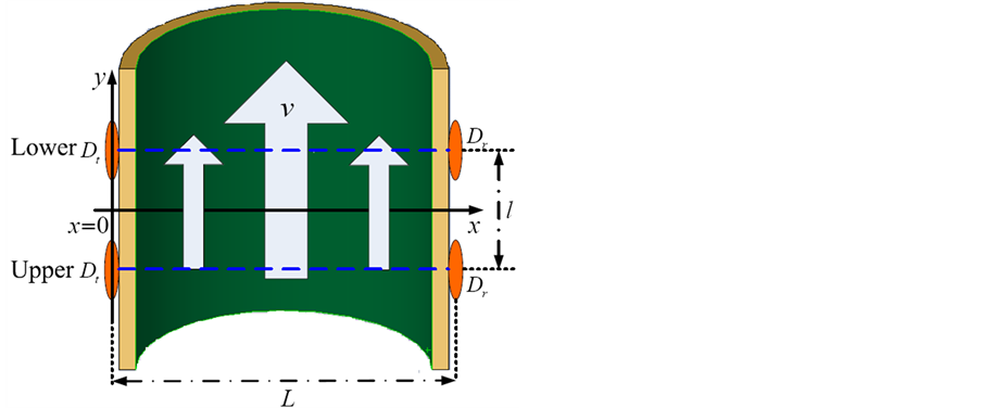
Figure 1. Schematic diagram of GFVMS.
dies and small eddies dissipating as heat [11] . This process is called cascade model. Borrowing ideas from this theory, the distribution of particulate concentration in stack can also be divided into masses of different sizes. And the evolution of masses can be described as small masses integrating together and becoming larger masses gradually. This process can be described by an anti-cascade model shown in Figure 2.
The received light intensity after crossing gas flow can be expressed as [12] [13]
 . (1)
. (1)
where
 is the assemble average of light intensity, and
 is the perturbation of extinction coefficient. Then, the correlation function of
optical scintillations detected by two detectors is
is the perturbation of extinction coefficient. Then, the correlation function of
optical scintillations detected by two detectors is
 , (2)
, (2)
where
 is the time delay.
 and
and
 are points on upstream and downstream of optical paths, respectively. For homogeneous
isotropic stationary gas flow,
are points on upstream and downstream of optical paths, respectively. For homogeneous
isotropic stationary gas flow,
 . (3)
. (3)
Based on the geometrical relationship in Figure 1 and the Taylor frozen hypothesis for turbulence,
 . (4)
. (4)
 is an even function, so
 . (5)
. (5)
The gas flow is homogeneous isotropic stationary, so the correlation function of
 can be expressed as
 . (6)
. (6)
After substituting
 with
with , function (6) can be written as
 . (7)
. (7)

Figure 2. Anti-cascade model for evolution of particulate concentration distribution.
 and
and
 are inner and outer scales of pieces mentioned in anti-cascade model, and
 is structure constant. When
 ,
, . Then, function (5) can be expressed
as
. Then, function (5) can be expressed
as
 , (8)
, (8)
Equation (8) illustrates that it is feasible to calculate gas flow velocity with the optical scintillation induced by fluctuation of particulate concentration.
3. Experimental Results
3.1. Experiments on Simulation Flue
In order to test the performance of GFVMS, a simulation flue is set up in laboratory, and its inner diameter and length are 32 cm and 12 m. A blower, the inner diameter and air displacement of which are 32 cm and 2.17 m3/s respectively, is placed at one end of the flue. A silicon controlled speed regulator is used to control the rotational speed of blower, and the velocity of gas flow can vary from 0 to 10 m/s. The GFVMS is installed at the other end of the flue. The distance between two probing beams is 30 cm (shown in Figure 3).
3.1.1. Comparison of Signals before and after Particles Added into Gas Flow
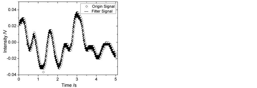
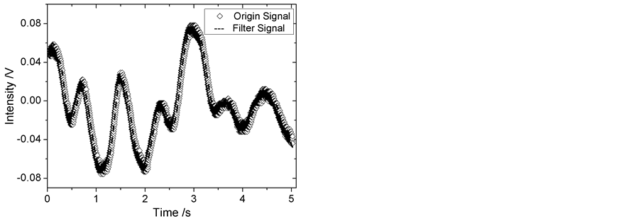
Before adding particles into gas flow, the temporal variations of signals after 450 times amplification are shown in Figure 4. In this picture, the straight and dotted lines are signals of channel A and B, respectively. Figure 5 is the temporal variations of signals after particles added into gas flow. In these figures, the rhombuses and dashed lines denote signals before and after 5 Hz low pass filter, respectively. The standard deviations of signals on two channels before adding particles are 1.98 mv and 4.32 mv. The values increase to 16.7 mv and 35.3 mv after particles added. These results indicate that, optical scintillations after adding particles are mainly induced by particulate concentration fluctuation.
In order to find out the reason why the amplitude of signal on channel B is rather large than that on channel A, two group ratios of standard deviations on channel B to the corresponding values on channel A are calculated. The data used here are selected randomly from experimental results before and after particles added. After given risen order of these ratios, a good linear fitting result is acquired (shown in Figure 6), the Adj. R-Square of which is 0.912. The distance between two probing beams is only 30 cm, so the particulate concentration transiting from upstream to downstream can’t change obviously [14] . Then, the only reasonable explanation for the difference of signal intensity is that channel B is more sensitive.
3.1.2. Determination of Particulate Concentration Ensuring GFVMS Work Stably
When particles are added into gas flow, continuous measuring results of velocities are shown in Figure 7. Synchronous variations of particulate number concentration measured by aerodynamic particle sizer of TSI (APS-3321) are shown in Figure 8. The preset velocity of gas flow confirmed by Pitot tube is about 3.5 m/s.
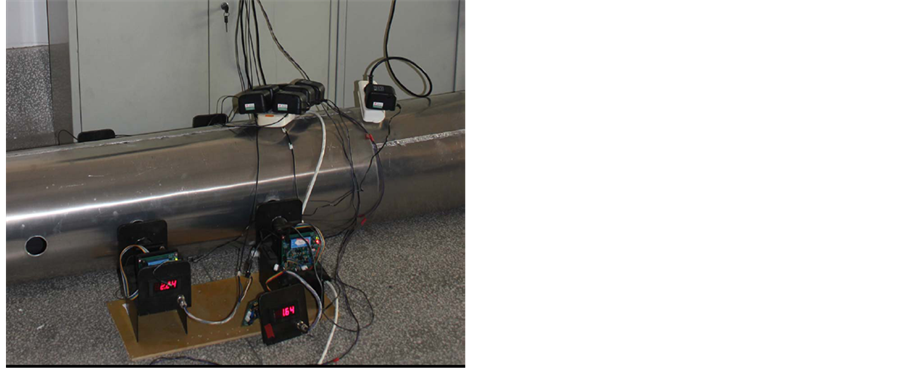
Figure 3. Picture of experiment on simulation flue.

Figure 4. Temporal variations of signals before particles added into gas flow.
 (a)
(a)
 (b)
(b)
Figure 5 Temporal variation of signals after particles added into gas flow. (a) Signal on channel A; (b) Signal on channel B.
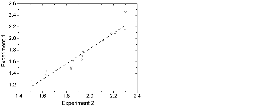
Figure 6. Linear fitting result for ratios of standard deviation.
Before adding particles, the GFVMS can’t work stably, and the measurement results are not accordance with the preset velocity. When particles are added, particulate number concentration increases rapidly [15] [16] . About 30 seconds later, the particulate number concentration reaches 4000/cm3, and the GFVMS can work stably. The
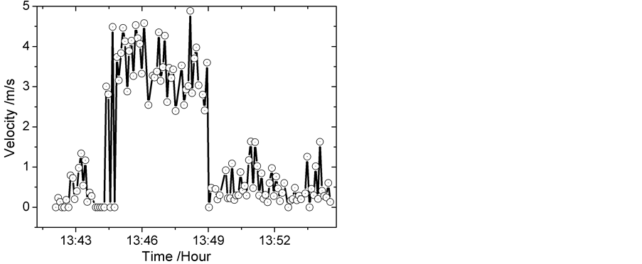
Figure 7. Temporal variation of gas flow velocity.

Figure 8. Temporal variation of particulate number concentration.
measured velocities vary among 3 - 4 m/s. When we stop adding particles, the particulate number concentration decreases gradually. If particulate number concentration is lower than 4000/cm3, unreasonable measurement results arise at once. That is, for this kind of particles, 4000/cm3 is the threshold of particulate number concentration, beyond which the GFVMS can work stably. The experiment is carried out in our lab, and the flue gas mixed with particles is discharged into the lab directly. So when stop adding particles, decrease process takes more time than the increase process for the same variation range of particulate number concentration.
3.1.3. Sensitivity Test
In order to test the sensitivity of GFVMS to velocity change, another experiment is carried out in which the gas flow velocity is increased from about 3 m/s to about 4.5 m/s. Velocities measured by GFVMS are shown as straight line in Figure 9. Synchronous results measured by Pitot tube CP 300 [17] are shown as actual velocity (dashed line in Figure 9). Before changing gas flow velocity, results measured by GFVMS and Pitot tube are both varying from 2.5 to 3.5 m/s. When flue gas velocity changed suddenly, velocities measured by GFVMS increase gradually. About 10 s (about 2 group data) later, results measured by two equipments converge to about 4.5 m/s, which indicate that the GFVMS is sensible to velocity change.
3.2. Outfield Testing Experiment
In order to test the practicality of GFVMS, outfield experiment is carried out on an industrial stack located at Shouguang, Shandong province of China. The cross section of the stack is rectangle, and its length and width are 1.5 m and 0.6 m, respectively. Figure 10 is the picture of outfield experiment. The distance between two probing beams is 0.3 m, and the sampling frequency is set to 2500 Hz.
Variation of gas flow velocities measured by GFVMS on industrial stack is shown in Figure 11, and Figure 12 is that measured by Pitot tube. The average velocity measured by GFVMS is 7.62 m/s, which is very close to that (8.30 m/s) measured by Pitot tube. That is, the GFVMS can measure gas flow velocity on industrial stack efficiently. However, the velocities measured by GFVMS are more stable comparing to those of Pitot tube. The main reasons induced this difference are given as follows. a) The difference may be caused by the unsynchronized measurement. There are only 2 pairs of hole on stack, so the GFVMS and Pitot tube can’t work synchronously. Thus, velocities shown in Figure 11 are measured during the first night, and velocities in Figure 12 are measured during the second night. b) Measurement results of GFVMS are average velocities along the optical path, but velocities measured by Pitot tube are those at a single point. c) Pitot tube belongs to invasive measurement and the instrument itself may change velocities near measurement point.
To analyze the spatial distribution of velocities in industrial stack and its influence to average velocity, velocities at different positions along the optical path of GFVMS are measured point-to-point using Pitot tube. The first point is 5 cm away from the wall of stack, and the distances of adjacent measurement points are all 10 cm. Measurement results are shown in Figure 13, where diamonds are real-time velocities measured at each point,
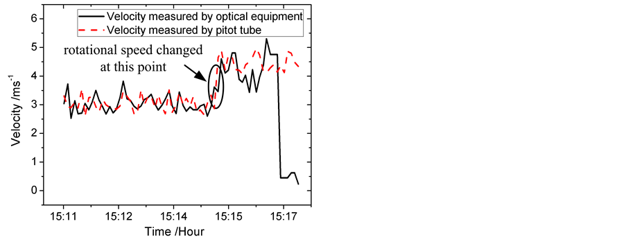
Figure 9. Measurement results when gas flow velocity changed suddenly.
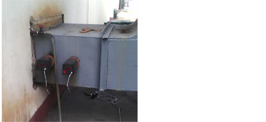
Figure 10. Picture of outfield experiment.
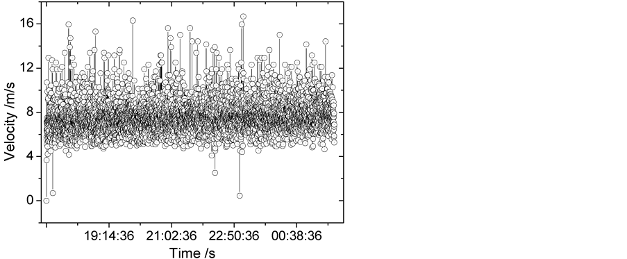
Figure 11. Temporal variation of gas flow.
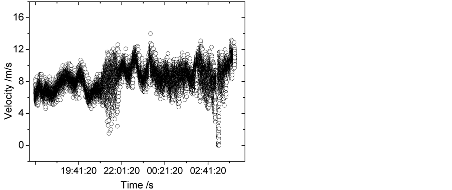
Figure 12. Temporal variation of gas flow velocities measured by Pitot tube.

Figure 13. Spatial distribution of gas flow velocity in industrial stack.
and triangles represent average velocities. For the existence of blower near the entrance of stack, spatial distribution of velocities is similar to the letter m. The average velocity of different measurement points is 7.61 m/s, which is identical with that measured by GFVMS. This result confirms the correctness of measurement results by GFVMS.
4. Conclusion
When particulate concentration in gas flow exceeds the needed threshold, the GFVMS can work normally, and the measurement results of GFVMS are identical with those of Pitot tube. Meanwhile, the results of sensitivity test indicate that GFVMS is very sensitive to velocity change. For the influence of several factors mentioned in our paper, the average velocity measured by GFVMS on industrial stack is smaller than that measured by Pitot tube at a single point. But the statistical average of velocities measured by Pitot tube at different points along the optical path is identical with average velocity measured by GFVMS. That is, measurement results of GFVMS can give us a better understanding of industrial emissions. In the future, we need more outfield experiments to test the performance of GFVMS and the data proceeding method.
References
- Andersson, B.J. (1958) On Measurement of Velocity by Pitottube. Arkivfor Matematik, 3, 391-394.http://dx.doi.org/10.1007/BF02589492
- Stainback, P.C. and Nagabushana, K.A. Review of Hot-Wire Anemometry Techniques and the Range of Their Applicability for Various Flows. Electronic Journal of Fluids Engineering, 1-54.
- Denham, M.K., Briard, P. and Patrick, M.A. (1975) A Directionally-Sensitive Laser Anemometer for Velocity Measurements in Highly Turbulent Flows. Journal of Physics E: Scientific Instruments, 8, 681-683.http://dx.doi.org/10.1088/0022-3735/8/8/019
- Wang, T.-I., Ochs, G.R. and Lawrence, R.S. (1981) Wind Measurements by the Temporal Cross-Correlation of the Optical Scintillations. Applied Optics, 20, 4073-4081. http://dx.doi.org/10.1364/AO.20.004073
- Wang, T.-I. (2002) Optical Flow Sensor. USA Patent No. 6,369,881 B1.
- Tatarskii, V.I. (1961) Wave Propagation in Turbulent Medium. McGraw-Hill, New York.
- Chen, A.S., Hao, J.M., Zhou, Z.P., et al. (1999) Theoretical Solutions for Particulate Scintillation Monitors. Optics Communications, 166, 15-20. http://dx.doi.org/10.1016/S0030-4018(99)00271-0
- Chen, A.S., Hao, J.M., Zhou, Z.P., et al. (2000) Particulate Concentration Measured from Scattered Light Fluctuations. Optics Letters, 25, 689-691. http://dx.doi.org/10.1364/OL.25.000689
- Chen, A.S., Hao, J.M., Zhou, Z.P., et al. (2000) Measuring Particulate Concentration by Means of Scattered Light Scintillation. SPIE Proceeding, 4222, 71-75.
- Ralph, L., Roberson, G., Clark, M., et al. (1997) Evaluation of Continuous Particulate Matter (PM) Monitors for Coal-Fired Utility Boilers with Electrostatic Precipitators. http://rmb-consulting.com/denpaper/rlrdenpa.htm
- Rao, R.-Z. (2005) Light Propagation in the Turbulent Atmosphere. Anhui Science & Technology Publishing House, Hefei.
- El-Wakil, S.A., Elgarayhi, A. and Elhanbaly, A. (2005) Transmission of Radiation through an Aerosol Medium. Journal of Quantitative Spectroscopy & Radiative Transfer, 93, 521-530. http://dx.doi.org/10.1016/j.jqsrt.2004.10.005
- Chamaillard, K., Kleefeld, C., Jennings, S.G., et al. (2006) Light Scattering Properties of Sea-Salt Aerosol Particles Inferred from Modeling Studies and Ground-Based Measurements. Journal of Quantitative Spectroscopy & Radiative Transfer, 101, 498-511. http://dx.doi.org/10.1016/j.jqsrt.2006.02.062
- Li, X.B., Xu, C.D., Luo, J., et al. (2009) Analysis on Two Methods of Measuring Refractive Index of Aerosol Particles. China Powder Science and Technology, 15, 72-74. (in Chinese)
- Huang, Y.-B., Huang, H.-L., Han, Y., et al. (2007) Measurement and Model Analysis of the Aerosol Optical Properties in the Regions of Hefei and Southeast Coast. Journal of Atmospheric and Environmental Optics, 2, 423-433. (in Chinese)
- Ministry of Environmental Protection (1997) Integrated Emission Standard of Air Pollutants. Integrated Emission Standard of Air Pollutants GB16297-1996. (in Chinese)
- KIMO Instrument (2007) CP 300 Operation Manual: Setting of 300 Series Transducer.
NOTES

*Corresponding author.