World Journal of Mechanics
Vol. 1 No. 3 (2011) , Article ID: 5780 , 10 pages DOI:10.4236/wjm.2011.13021
A Simplified Nonlinear Generalized Maxwell Model for Predicting the Time Dependent Behavior of Viscoelastic Materials
Département de Physique, Université d’Abomey-Calavi, Abomey-Calavi, Bénin
E-mail: monsiadelphin@yahoo.fr
Received April 13, 2011; revised May 12, 2011; accepted May 23, 2011
Keywords: Hyperlogistic-Type Function, Maxwell Model, Nonlinear Stress-Time Relationship, Riccati Equation, Viscoelasticity
ABSTRACT
In this paper, a simple nonlinear Maxwell model consisting of a nonlinear spring connected in series with a nonlinear dashpot obeying a power-law with constant material parameters, for representing successfully the time-dependent properties of a variety of viscoelastic materials, is proposed. Numerical examples are performed to illustrate the sensitivity of the model to material parameters.
1. Introduction
To better understanding mechanical responses of materials subjected to deformations or forces, theoretical models are required. These models provide important analytical tools for predicting and simulating material functions. When a material is subjected to deformations, the resulting stress is related to the strain by a mathematical relationship known as the constitutive law. This constitutive equation can, thus, provide usefulness in determining rheological properties of materials. Since viscoelastic materials exhibit both combined viscous and elastic material behaviors, their constitutive equation must mathematically relate stress, strain and their time derivatives. For this purpose, these constitutive equations are often determined from combinations of springs and dashpots arranged in series and/or parallel [1]. Since mechanical responses of viscoelastic materials are in general nonlinear, the well-known established linear theory of viscoelasticity must be reasonably replaced by nonlinear theories. But, nonlinear models are more difficult to formulate than linear theories, because these models lead often to solve nonlinear differential equations that are generally non-integrable. In this perspective, several models of different complexities have been proposed to describe viscoelastic material functions [2]. To take into account nonlinear viscoelastic material properties, it is needed to modify the simple classical Maxwell and Voigt models or their different combinations for including nonlinear terms. Many successful predictive models are shown to be based on the extension of classical linear rheological models to finite deformations [3] and “in press” [4-8]. The modifications consist to introduce nonlinear elastic springs and/or nonlinear dashpots in the classical linear models. Another way is to consider that the materials functions depend on the magnitude of the stress, strain or the strain rate. The resulting model according to Alfrey and Doty [1], is interesting since, it evaluates the material properties in terms of differential equations that can be solved for a wide variety of transient conditions. In viscoelasticity theory, there are only a few theoretical models formulated with constant-value material coefficients [3]. Thus, constant coefficients nonlinear rheological models are required. Following this viewpoint, Corr et al. [3] extending the Maxwell fluid model to finite deformations, constructed a Riccati differential equation that is useful to describe the strain stiffening and softening response of some viscoelastic materials. Recently, Monsia “in press” [4] utilizing a power series expansion method that consisted in an extended Voigt model to large deformations taking into consideration the inertia term, developed a hyperlogistic equation which represents successfully the timedependent mechanical properties, that is to say, the strain stiffening and softening behavior, of a variety of viscoelastic materials. Recently again, Monsia “in press” [5] using a second-order elastic spring in series with a classical Voigt element, which is an extended form of the standard linear solid to finite strains, formulated a hyperlogistic-type equation to reproduce the nonlinear time-dependent stress response of some viscoelastic materials. More recently, Monsia “in press” [6] developed a single differential constitutive equation derived from a standard nonlinear solid model consisting of a polynomial elastic spring in series with a classical Voigt element for the prediction of time- dependent nonlinear stress of a class of viscoelastic materials. More recently again, Monsia “in press” [7] formulated a nonlinear four-parameter rheological Voigt model consisting of a nonlinear Voigt element in series with a classical linear Voigt element with constant material coefficients for representing the nonlinear stiffening response of the initial low-load portion and the softening, that is to say, the S-shaped mechanical behavior of some viscoelastic materials. Very lately, Monsia “in press” [8] generalized successfully the previous model “in press” [7] by replacing the second-order elastic spring present in the nonlinear Voigt element by a polynomial elastic spring. The model “in press” [8] was shown to be able to predict accurately the nonlinear stiffening response of the initial low-load portion and the softening behavior of a variety of viscoelastic materials.
In this study, a simple nonlinear Maxwell model (Figure 1) consisting of a nonlinear spring connected in series with a nonlinear dashpot obeying a power-law with constant material parameters, for representing successfully the time-dependent properties of a variety of viscoelastic materials, is proposed. Under a linear strain-path control the constitutive law gives a mathematical description of the stress versus time relationship as a hyperlogistic function, which appears powerful to represent any S-shaped curve. The model can then correctly reproduce the strain stiffening and softening responses noted in some viscoelastic materials at large strains. Numerical examples are performed to illustrate the sensitivity of the model to material coefficients and the validity of the model. In particular the model is shown to be very sensitive to the magnitude of the rate of application of the strain.

Figure 1. The proposed rheological model.
2. Mechanical Model
2.1. Theoretical Formulation
In this part we describe the theoretical rheological model and derive the governing differential equation including the nonlinear restoring force and damping effects. Most viscoelastic materials are highly influenced by the nonlinear elastic and viscous damping terms so that, their rheological material properties are nonlinear timedependent. For this, a best description of these materials must proceed from the use of nonlinear theories. To build our proposed viscoelastic model, we start from the classical linear Maxwell model [1] in which we replace the linear elastic spring with a nonlinear elastic spring (with stiffness E) obeying a power-law and also the linear dashpot with a nonlinear dashpot (with viscosity η) obeying a power-law as shown in Figure 1. Thus, the mechanical properties of the considered material are divided into two parts: a nonlinear elastic element which captures the nonlinear pure elastic behavior of the material at equilibrium, acting in series with a nonlinear damping element capturing the time dependent history response of the material. From the mathematical point of view, the nonlinear stiffness and the nonlinear damping terms are included in a model in order to loss the linearity in the differential constitutive equation that represents the dynamic properties of the mechanical system studied. Due to the fact that the elements are in series the total stress  and the total strain
  can be written as
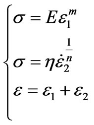 (1)
(1)
where  and
and  are the strains of the nonlinear spring and the nonlinear dashpot, respectively. η is the viscosity module, and E is the elasticity module. The dot denotes the time derivative and, m and n are nonlinearity parameters. By differentiations with respect to time and making appropriate substitutions, one can deduce from Equation (1) the constitutive differential equation
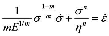 (2)
(2)
Equation (2) represents mathematically in the single differential form the relation between the total stress  induced in the material under a strain history
  . This equation is a first-order nonlinear ordinary differential equation in
  for a given strain history
  when the numbers m and n are identically different from the number one.
2.2. Dimensionalization
If  ,
,  and
and  denote the mass, length and time dimension, respectively, the dimension of the stress varies as
 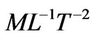 . The strain
  is a dimensionless quantity. Therefore, in Equation (2) the coefficient E possesses the same dimension with the stress
 , that of η varies as
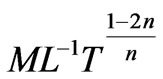 .
.
2.3. Solutions Using a Linear Strain-Path Control
We derive in this section the hyperlogistic-type solution allowing the description of the time-dependent stress induced in the material studied. For this, we consider that the material under consideration is subjected to a linear strain-path control, that is to say
 (3)
(3)
where  is the rate of application of the strain.
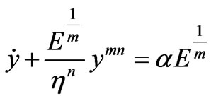
Thus, Equation (2) becomes
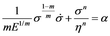 (4)
(4)
In order to solve Equation (4) we proceed to the following change of variable
 (5)
(5)
or
 (6)
(6)
Differentiating Equation (5) with respect to time yields
 (7)
(7)
Substituting these relationships (Equation (6) and (7)) into Equation (4), the resulting equation becomes
 (8)
(8)
Equation (8) is also a first-order ordinary differential equation in y, which can be solved analytically with the suitable boundary conditions of the mechanical problem considered in hyper-exponential or hyperlogistic-type function for special values of the exponent mn.
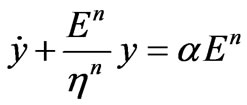
2.3.1. Case A: 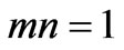
In this particular case where 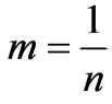 , Equation (8) becomes a simple linear first-order ordinary differential equation
 (9)
(9)
which can be easily solved analytically using the initial condition
 ,
, 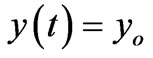
Thus, we can obtain as solution
 (10)
(10)
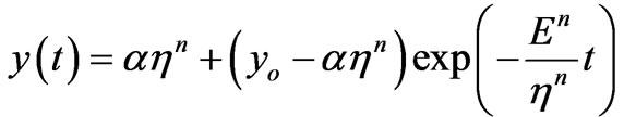
From the Equation (6) we may deduce taking into account the Equation (10) the stress versus time as
 (11)
(11)
Equation (11) gives the time variation of the stress in the viscoelastic material studied. It models the timedependent stress as a hyper-exponential function showing that the initial stress is different from zero. Moreover, Equation (11) predicts a stress that asymptotically approaches a maximum value with increasing time.
2.3.2. Case B: 
In this particular case where  , Equation (8) becomes a first-order Riccati nonlinear ordinary differential equation [3] and “in press” [4-8].
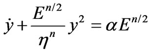 (12)
(12)
which can be easily solved analytically using the initial condition
 ,
, 
Therefore, we can obtain as solution
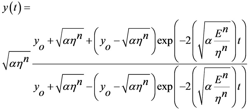 (13)
(13)
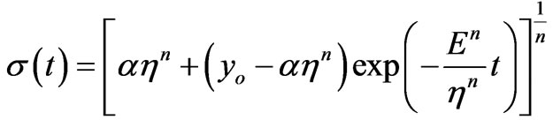
We can deduce from Equation (6) taking into consideration the above Equation (13) the stress versus time
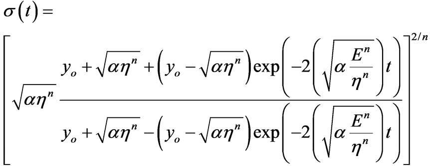 (14)
(14)
Equation (14) describes the time variation of the stress in the viscoelastic material studied as a hyperlogistic-type function, which is powerful to reproduce any S-shaped curve [9,10].
3. Numerical Results and Discussion
In this part some numerical examples concerning the time-dependent stress are presented to illustrate the ability of the model to reproduce the mechanical response of the viscoelastic material studied. The dependence of the stress versus time curve on the material parameters is also discussed.
3.1. Case A: 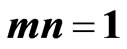
Figure 2 exhibits the typical time-dependent stress curve with an increasing until a peak asymptotical value, obtained from Equation (11) with the value of coefficients ,
,  ,
,  ,
,  ,
,  . It can be seen from Figure 2 that the model is capable to represent mathematically and accurately the typical exponential stiffening of some viscoelastic materials, for example, soft living tissues and soils, as shown in [3] and “in press” [4-8]. The model predicts a mechanical response in which the slope, after reaching its maximum value at the inflexion point, declines gradually with increase time until the failure point at which the slope reduces to zero.
Figure 3(a), (b), (c), (d) and (e) shows the effect of material parameters on the time-stress response. The effects of these parameters are studied by varying one coefficient while keeping the other four constant. Figure 3(a) illustrates how the rate of application of the strain  affects the maximum value of the stress. The graph shows that an increasing
 , increases the maximum stress and the slope, and has no significant effect on the time required to reach the maximum stress and on the initial value of the stress. The red color corresponds to
  , the blue to
  , and the green to
  . The other parameters are
  ,
,  ,
,  ,
,  .
.
In Figure 3(b) is shown the dependence of the stress on the viscosity coefficient η. An increase  , increases the peak stress and the time needed to reach it. The slope increases also. But an increasing η, has no important effect on the initial value of the stress. The red color corresponds to
  , the blue to
  , and the green to
  . The other parameters are
  ,
,  ,
,  ,
,  .
.
The stress curves at various values of the elasticity module E for the material under study are shown in Figure 3(c). An increasing E, greatly and fast increases the value of the stress on the time period considered. The slope increases with increase E. The red color corresponds to  , the blue to
  , and the green to
  . The other parameters are
  ,
,  ,
,  ,
,  .
.
Figure 3(d) shows the sensitivity of the stress-time curve to the nonlinearity parameter n. An increasing nonlinearity parameter n, has a high effect on the stress value in the time period considered. Indeed, an increasing n, significantly and fast increases the value of the stress and also the initial value of the stress increases with increase n. The red color corresponds to  , the blue to
  , and the green to
  . The other parameters are
  ,
,  ,
,  ,
,  .
.
We observe from Figure 3(e) that an increasing initial value , has a significant effect on the stress value in the time period considered. In fact, an increase
 , increases significantly and fast the stress value and also the initial value of the stress. An increasing
 , reduces the slope. The stress becomes constant, that is to say,

or
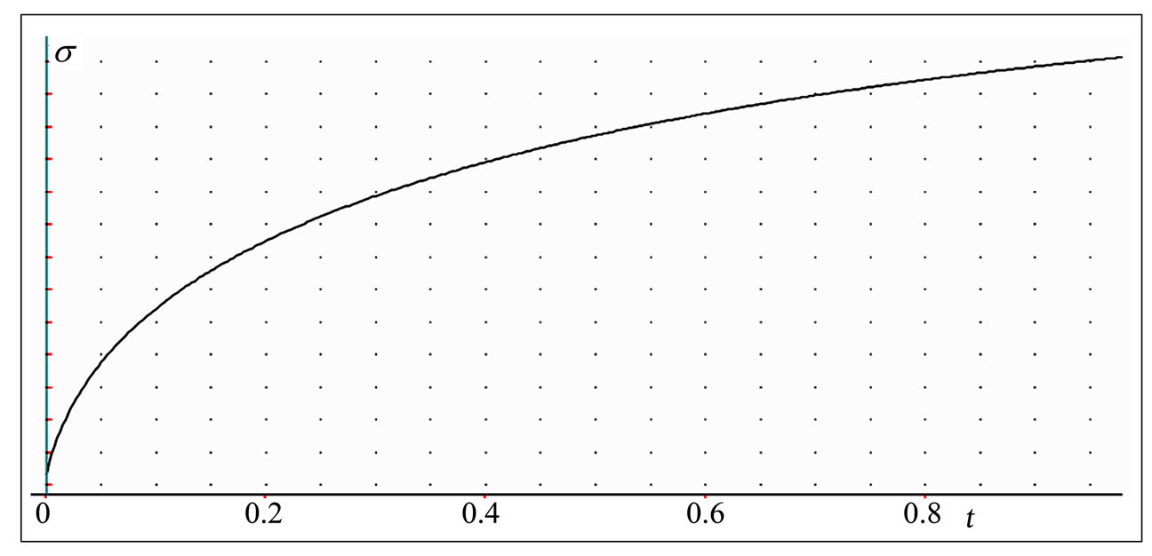
Figure 2. Typical stress-time plotting exhibiting a maximum asymptotical value.
 (a)
(a)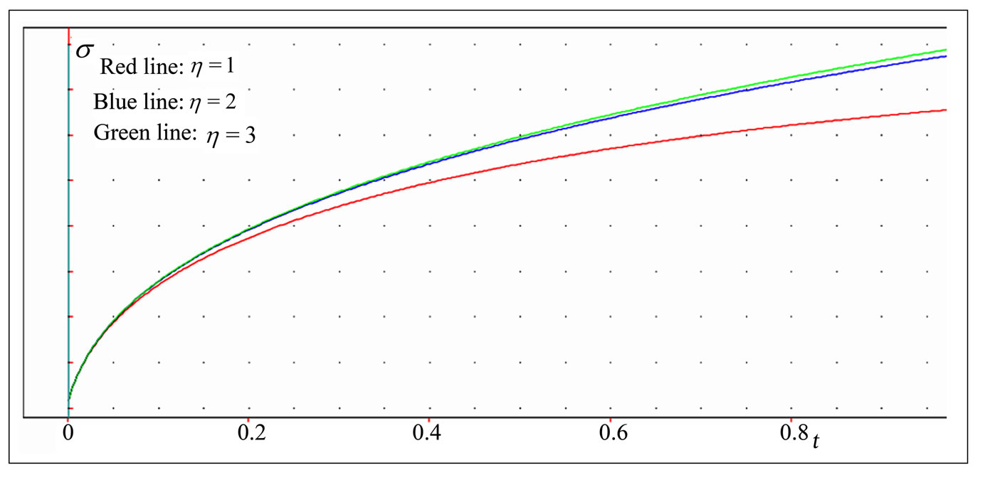 (b)
(b)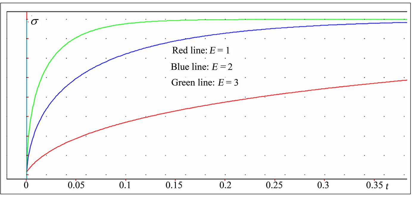 (c)
(c)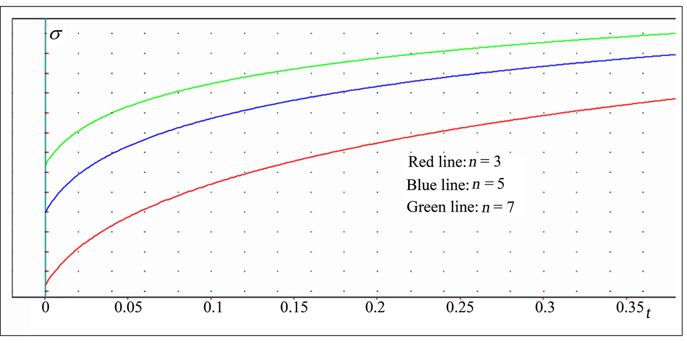 (d)
(d)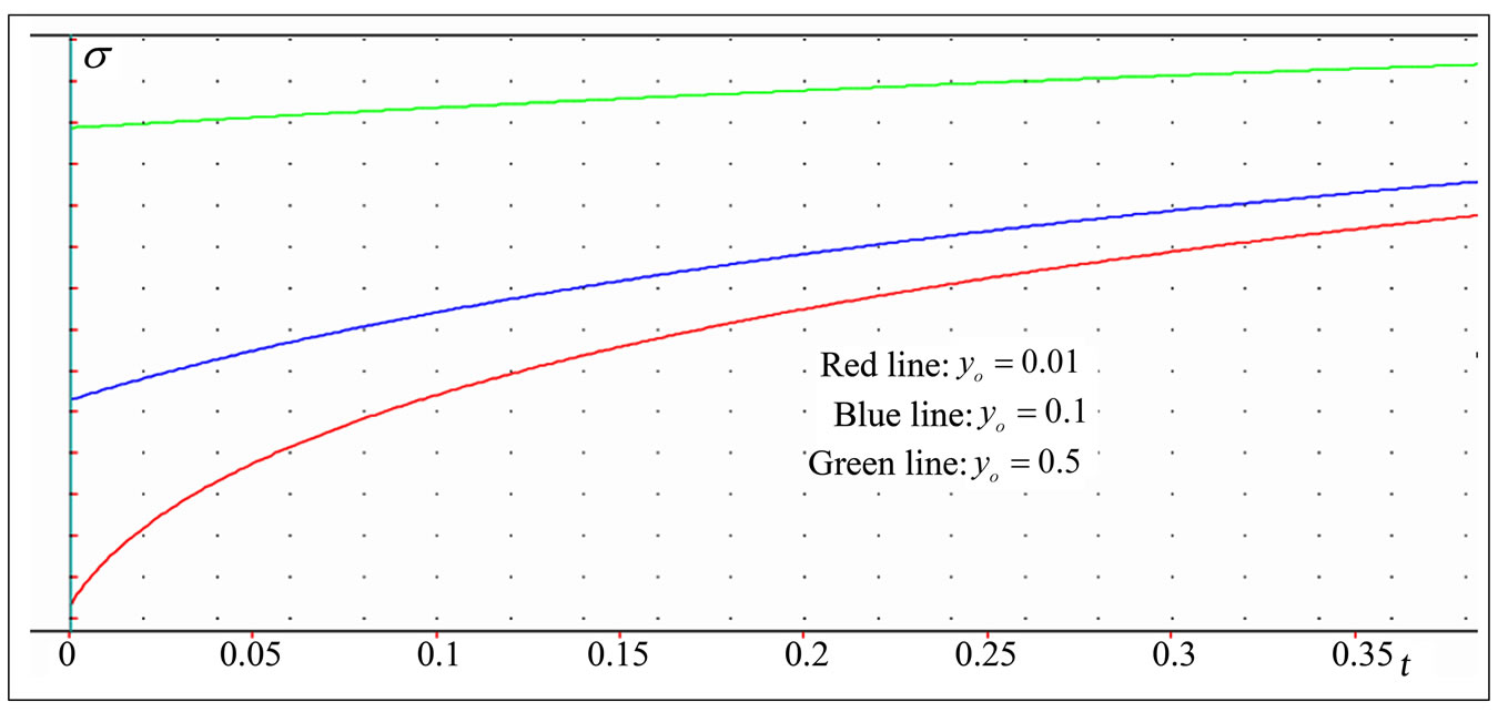 (e)
(e)
Figure 3. (a). Stress versus time curves at various values of the strain rate; (b). Stress-time curves with different values of the viscosity module; (c). Stress versus time curves showing the effect of the elasticity module E; (d). Stress versus time curves with different values of the nonlinearity parameter n; (e). Stress-time curves for three different values of .
.
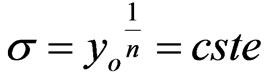
with
and the slope reduces to zero. The red color corresponds to  , the blue to
  , and the green to
  . The other parameters are
  ,
,  ,
,  ,
,  .
.
3.2. Case B: 
Figure 4 exhibits the typical time-dependent stress curve with an increasing until a peak asymptotical value, obtained from Equation (14) with the value of coefficients
 ,
,  ,
,  ,
,  ,
,  . It can be observed from Figure 4 that the model is able to represent accurately the typical time-dependent stress curve of a variety of viscoelastic materials, as mentioned above, for example, soft living tissues and soils, as shown in [3] and “in press” [4-8]. The stress versus time curve is nonlinear, with a nonlinear beginning initial portion, and illustrates then the sigmoid mechanical behavior of the viscoelastic material considered. The plotting showing a nonlinear sigmoid behavior indicates, consequently, the material stiffening followed by softening. The model predicts a mechanical response in which the slope, after reaching its maximum value at the inflexion point, declines gradually with increase time until the failure point at which the slope reduces to zero.
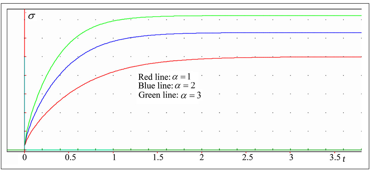
In Figure 5(a) is shown the dependence of the stress versus time curve on the strain rate . The graph indicates that the peak stress increases with increasing
  . The slope increases also with increase the rate of application of the strain. But, an increasing
 , has no important effect on the time required to attain the peak stress. The red color corresponds to
  , the blue to
  , and the green to
  . The other parameters are
  ,
,  ,
,  ,
,  .
.
Figure 5(b) illustrates how the viscosity coefficient η
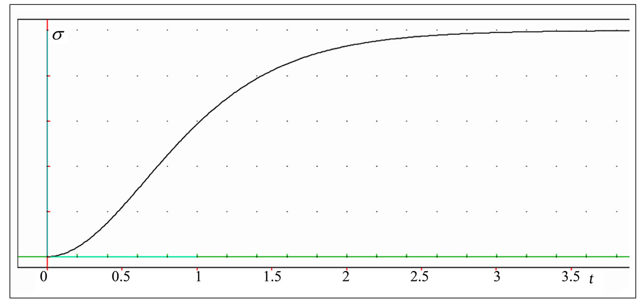
Figure 4. Typical stress versus time curve exhibiting a maximum asymptotical value.
 (a)
(a)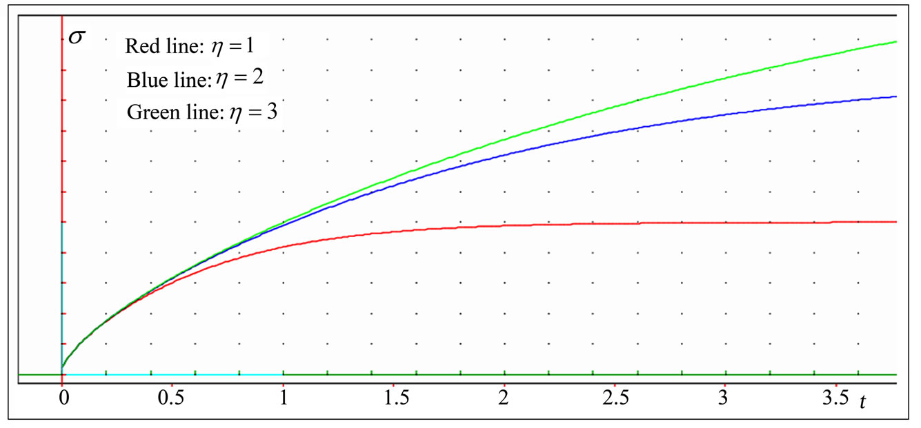 (b)
(b)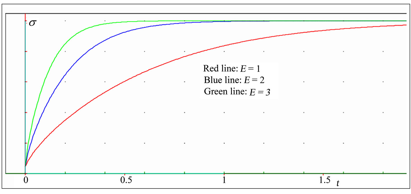 (c)
(c)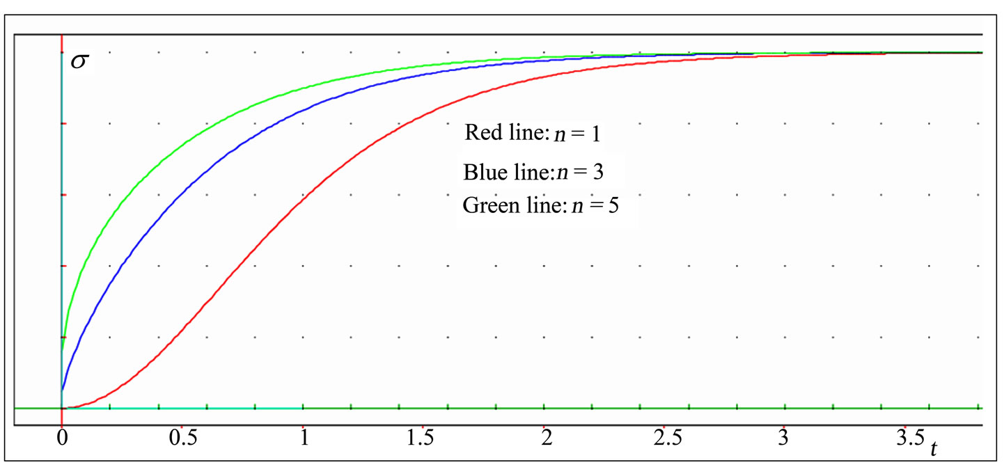 (d)
(d)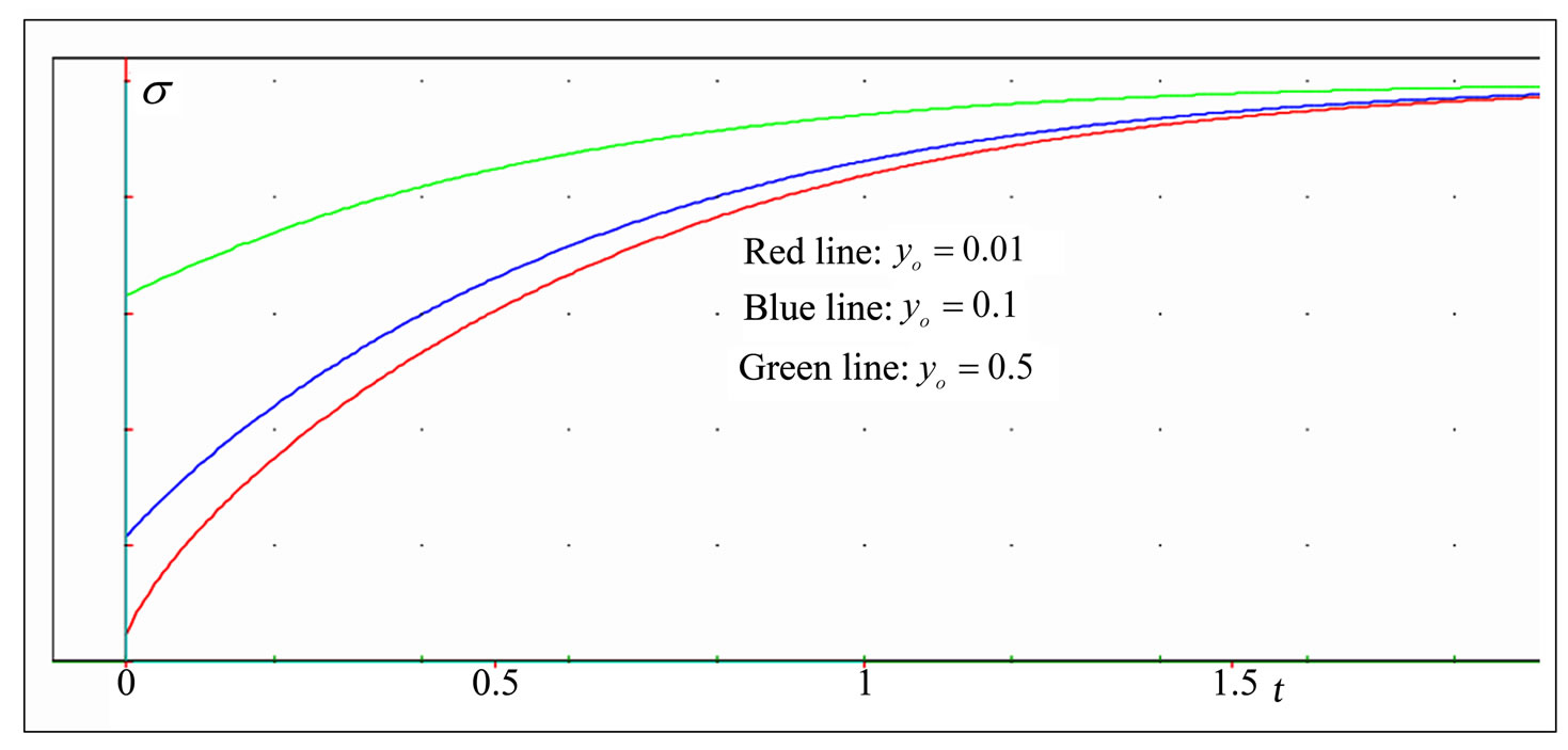 (e)
(e)
Figure 5. (a). Stress-time curves at various values of the rate of application of the strain  . (b). Stress versus time curves at three different values of the coefficient of viscosity η. (c). Stress-time curves for various values of the elasticity module E. (d). Stress-time curves showing the effect of the nonlinearity parameter n; (e). Stress versus time curves for three different values
  .
.
affects the maximum value of the stress. The graph shows that an increasing η, increases the maximum stress and increases also the time needed to attain the maximum stress. The red color corresponds to  , the blue to
  , and the green to
  . The other parameters are
  ,
,  ,
,  ,
,  .
.
It can be observed from Figure 5(c) the dependence of the stress on the elasticity module E. An increase E, has a great influence on the stress value. Indeed, it increases fast in the early periods of time. Then, this influence decreases as time tends to infinity, and the curves tend towards the same asymptotic value of the stress. The slope increases with increase E. The red color corresponds to  , the blue to
  , and the green to
  . The other parameters are
  ,
,  ,
,  ,
,  .
.
The stress curves at various values of the nonlinearity parameter n for the material under consideration are shown in Figure 5(d). An increasing n, has a high effect on the stress value. In fact, the stress increases fast in the early periods of time. Then, this effect decreases as time tends to infinity, and the curves tend towards the same asymptotic value of the stress. The nonlinearity of the initial portion of curves becomes less important with increasing n. The red color corresponds to  , the blue to
  , and the green to
  . The other parameters are
  ,
,  ,
,  ,
,  .
.
We observe from Figure 5(e) that an increasing initial value  , has an important effect on the stress value. Indeed, the stress increases fast in the early periods of time. Then, this influence decreases as time tends to infinity, and the curves tend towards the same asymptotic value of the stress. Moreover, an increasing
  , increases the initial value of the stress. The red color corresponds to
  , the blue to
  , and the green to
  . The other parameters are
  ,
,  ,
,  ,
,  .
.
The previous numerical examples show that theoretical models are important tools for the prediction and simulation of viscoelastic behavior of materials. In this work, a simple nonlinear viscoelastic model is presented. The present model has been developed following two working hypothesis. The first postulates that the material properties can be divided into a nonlinear pure elastic component obeying a power-law and acting in series with a nonlinear damping element obeying a power-law and capturing the time-dependent deviation from the equilibrium state. The second hypothesis assumes that the material is subjected to a linear strain-path control. Under these restrictions, the model predicted the timedependent stress induced in the material as a hyperlogistic-type function, which is able to reproduce any S-shaped curve as shown by numerical examples. These predicted results by the proposed model are in very agreement with those published in the literature. The proposed model is an extension of the classical Maxwell model to large deformations by means of two parameters m and n. It appeared evident that for  and
and  , the present model reduces to the well-known Maxwell model. Consequently, these parameters assure the role of nonlinearity coefficients.
4. Conclusions
A complete characterization of viscoelastic materials is very difficult to perform, due to the fact that the mechanical response of these materials is time-dependent and history-dependent, and moreover, their stress-strain curve is nonlinear. Following this viewpoint, nonlinear theoretical models are necessary to better predict and understand the time-dependent behavior of materials. For this purpose, a nonlinear generalized Maxwell model has been developed. The model allowed, according to the obtained results, describing mathematically and accurately the nonlinear time-dependent stress in some viscoelastic materials, as a hyperlogistic-type function, that is powerful to represent any sigmoid curve. The present model, in particular, is shown to be very sensitive to the magnitude of the strain rate. Altogether, more experimental results and practical tests are needed to further validate the feasibility of this model.
REFERENCES
- T. Alfrey and P. Doty, “The Methods of Specifying the Properties of Viscoelastic Materials,” Journal of Applied Physics, Vol. 16, No. 11, 1945, pp. 700-713. doi:10.1063/1.1707524
- R. Chotard-Ghodsnia and C. Verdier, “Rheology of Living Materials,” In: F. Mollica, L. Preziosi and K. R. Rajagopal, Eds., Modeling of Biological Materials, Springer, New York, 2007, pp. 1-31. doi:10.1007/978-0-8176-4411-6_1
- D. T. Corr, M. J. Starr, R. Vanderby, Jr and T. M. Best, “A Nonlinear Generalized Maxwell Fluid Model for Viscoelastic Materials,” Journal of Applied Mechanics, Vol. 68, No. 5, 2001, pp. 787-790. doi:10.1115/1.1388615
- M. D. Monsia, “Lambert and Hyperlogistic Equations Models for Viscoelastic Materials: Time-Dependent Analysis,” International Journal of Mechanical Engineering, Serials Publications, New Delhi, India, January-June 2011.
- M. D. Monsia, “A Hyperlogistic-Type Model for the Prediction of Time-Dependent Nonlinear Behavior of Viscoelastic Materials,” International Journal of Mechanical Engineering, Serials Publications, New Delhi, India, January-June 2011.
- M. D. Monsia, “A Nonlinear Generalized Standard Solid Model for Viscoelastic Materials,” International Journal of Mechanical Engineering, Serials Publications, New Delhi, India, January-June 2011.
- M. D. Monsia, “A Modified Voigt Model for Nonlinear Viscoelastic Materials,” International Journal of Mechanical Engineering, Serials Publications, New Delhi, India, January-June 2011.
- M. D. Monsia, “A Nonlinear Generalized Four-parameter Voigt Model for Viscoelastic Materials,” International Journal of Mechanical Engineering, Serials Publications, New Delhi, India, July-December 2011.
- C. Debouche, “Présentation Coordonnée de Différents Modèles de Croissance, ” Revue de Statistique Appliquée, Vol. 27, No. 4, 1979, pp. 5-22. http://www.numdam.org/item?id=RSA_1979_27_4_5_0>
- O. Garcia, “Unifying Sigmoid Univariate Growth Equations,” Forest Biometry, Modelling and Information Sciences, Vol. 1, 2005, pp. 63-68. http://www.fbmis.info/A/5.1.GarciaO.1.pdf