Journal of Signal and Information Processing
Vol.4 No.3(2013), Article ID:36072,7 pages DOI:10.4236/jsip.2013.43042
Parametrically Optimal, Robust and Tree-Search Detection of Sparse Signals
![]()
1Oklahoma State University, Computer Science Department, Stillwater, USA; 2University of Colorado Denver, Electrical Engineering Department, Denver, USA.
Email: tburrell@okstate.edu, titsa.papantoni@ucdenver.edu
Copyright © 2013 A. T. Burrell, P. Papantoni-Kazakos. This is an open access article distributed under the Creative Commons Attribution License, which permits unrestricted use, distribution, and reproduction in any medium, provided the original work is properly cited.
Received June 30th, 2013; revised July 30th, 2013; accepted August 13th, 2013
Keywords: Sparse Signals; Detection; Robustness; Outlier Resistance; Tree Search
ABSTRACT
We consider sparse signals embedded in additive white noise. We study parametrically optimal as well as tree-search sub-optimal signal detection policies. As a special case, we consider a constant signal and Gaussian noise, with and without data outliers present. In the presence of outliers, we study outlier resistant robust detection techniques. We compare the studied policies in terms of error performance, complexity and resistance to outliers.
1. Introduction
In recent years, some refreshed interest has been given to sparse signals, by the signal processing community [1,2], while the effective probing/transmission of such signals; previously denoted bursty, has been addressed by both tree-search [3,4], and random access algorithms [5]. The revisited investigation of sparse signals has focused on linear transformations [1,2], while the term robustness has been used loosely in [1].
In this paper, we focus on the detection of sparse signals embedded in white Gaussian noise with the possible occasional occurrence of data outliers. We study both optimal and sub-optimal detection techniques, when data outliers are considered both absent and present. In the latter case, we consider robust detection techniques, where robustness is here precisely defined as referring to outlier resistant operations [6,7]. We compare our techniques in terms of error performance, complexity and resistance to outliers.
The organization of the paper is as follows: In Section 2, we state the fundamental general problem, present assumptions and notation, and determine, as well as partially analyze, the general optimal detector. In Section 3, we present and analyze the optimal detector for the case of white Gaussian noise and constant signal, when no outliers are considered in the design. In Section 4, we present and analyze the robust (outlier resistant) detector. In Section 5, we present and evaluate tree-search suboptimal detectors. In Section 6, we include discussion and conclusions.
2. Problem Statement and General Solution
We consider a sequence of observations generated by mutually independent random variables, a small percentage of which represent signal embedded in noise, while the remaining percentage represent just noise. Let it be known that the percentage of observations representing signal presence is bounded from above by a given value α. We assume that the random variables representing the signal are identically distributed, and that so are those representing the noise. We denote by , a sequence of n such observations, while we denote by
 , the sequence of mutually independent random variables whose realization is the sequence
 . We also denote by f1(.) either the probability distribution (for discrete variables) or the probability density (for absolutely continuous variables) function (pdf) of the variables which represent signal presence, while we denote by f0(.) the pdf of the variables which represent just noise.
Given the observation sequence  and assuming f1(.), f0(.), a known, the objective is to identify the locations of the signal presence; that is, which ones of the
  observations originated from the f1(.) pdf.
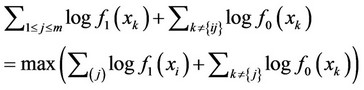
Our approach to the problem solution will be Maximum Likelihood (ML); which is equivalent to that of the Bayesian minimization of error probability approach, when all signal locations and their number are equally probable [7]. That is, given the sequence , the optimal detector decides in favor of the
 ; 0 £ m £ an signal locations if:
 (1)
(1)
Let us define:
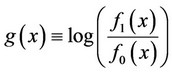 (2)
(2)
Via some straight forward modifications of the expression in (1), we may then express the optimal ML detector as follows:
Optimal ML Detector 1) Given the sequence , compute all g(xj); 1 £ j £ n 2) If g(xk) £ 0; for all k, 1 £ k £ n, then, decide that no observation contains signal.
3) If $ a set of integers ; 1 £ m £ an: g(xk) > 0; for all
  and g(xk) £ 0; for all
 , then decide that the observations containing the signal are all those with indices in the set
 .
.
4) If $ a set of integers ; m > an: g(xk) > 0; for all
  and g(xk) £ 0; for all
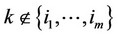 , then decide that the observations containing the signal are those whose indices k are contained in the set
  and whose g(xk) values are the an highest in the set.
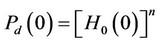
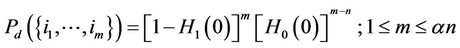
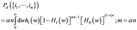
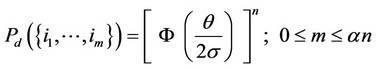
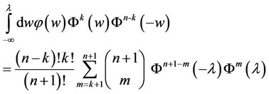
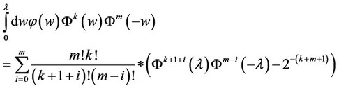
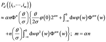
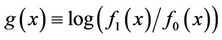
Considering the log likelihood ratio in (2), let hi(w) and Hi(w); i = 0, 1, denote, respectively, the pdf and the cumulative distribution function of the random variable g(X) at the value point w, given that the pdf of X is fi, i = 0, 1. Let Pd(0) denote the probability of correct detection induced by the optimal ML detector, given that no observation contains signal. Let, instead, 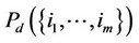
denote the probability of correct detection , given that the indices of the observations containing signal are given by the set . Then, assuming absolutely continuous {Xi} random variables; without lack in generality, we obtain the following expressions; without much difficulty, where an is assumed an integer; for simplicity in notation:
 (3)
(3)
Remarks It is important to note that the optimal detector presented above assumes no knowledge as to any structure of the sparse signal and requires n-size memory, as well as ordering of the positive g(xk) values, inducing complexity of order nlogn. If, on the other hand, a structure of the signal is known a priori and is such that it appears as a bursty batch, then, the sequential algorithm in [7-9] that monitors changes in distribution should be deployed instead; it requires no memory and its complexity is of order n.
3. Constant Signal and White Gaussian Additive Noise
In this section, we consider the special case where the signal is a known constant q > 0, and the noise is zero mean white Gaussian with standard deviation s. After some simple straight forward normalizations, the optimal ML detector of Section II takes here the lollowing form:
Optimal ML Detector 1) Given the sequence , compute all (xi – q/2); 1 £ j £ n 2) If (xk – q/2) £ 0; for all k, 1 £ k £ n, then, decide that no observation contains signal.
3) If $ a set of integers ; 1 £ m £ an: (xk – q/2) > 0; for all
  and (xk – q/2) £ 0; for all
 , then decide that the observations containing the signal are all those with indices in the set
 .
.
4) If $ a set of integers ; m > an: (xk – q/2) > 0; for all
 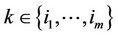 and (xk – q/2) £ 0; for all
 , then decide that the observations containing the signal are those whose indices k are contained in the set
  and whose (xk – q/2) values are the an highest in the set.
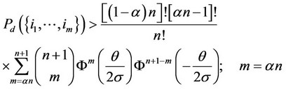
As to the probabilities of correct detection, defined in Section 2, they take the following form here, where j(x) and F(x) denote, respectively, the pdf and the cumulative distribution function of the zero mean and unit variance Gaussian random variable and where αn is assumed again to be an integer :
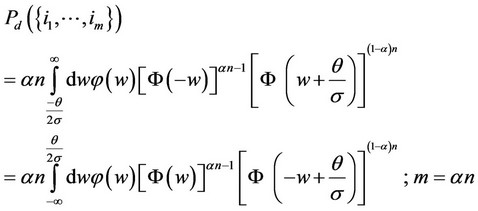 (4)
(4)
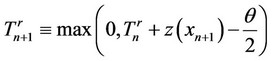
Remarks It is interesting to note here that if it is known that the signal may appear as a set bursty batches of unknown sizes, then the re-initialization sequential algorithm in [8] will sequentially detect the beginning and the ending of each batch with minimal complexity, no memory requirements and with accuracy increasing with the signal-to-noise ratio and the size of each batch. Let then Tn denote the value of the algorithm which detects the beginning of such a batch, upon the processing of the nth datum xn from its beginning. Let Wn denote the value of the algorithm which detects the ending of the batch, upon processing the nth datum yn from the beginning of its initialization. The whole algorithmic system operates then as follows, where d0 and d1 are two positive thresholds pre selected to satisfy power and false alarm trade offs:
1) Process the observed sequence  sequentially starting with the algorithm {Tn} whose values are updated as follows:

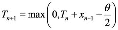
Stop the first time n, such that Tn ³ d0 and declare n as the time when the signal batch begins.
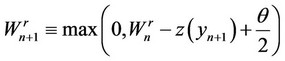
Then, switch immediately to the algorithm {Wn} whose values are updated as follows, where time zero denotes the time when the algorithm begins and where yn denotes the nth observed datum after the latter beginning:
2) 
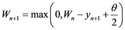
Stop the first time n, such that Wn ³ d1 and declare that the signal batch has ended.
We now express a Corollary which will be useful in the computation of bounds for the probability of correct detection in (4). The expressions in the Corollary are derived from recursive relationships produced via integration by parts and can be proven easily by induction.
Corollary The following equations hold:
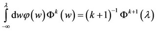 (5)
(5)
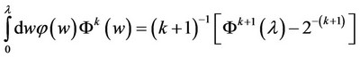 (6)
(6)
 (7)
(7)
 (8)
(8)
Lemma 1 below utilizes the results in the Corollary, to express two lower bounds for the probability of correct detection in (4). The bound in (9) is relatively tight for low signal-to-noise ratio values q/s. The bound in (10) is relatively tight for high signal-to-noise ratio q/s, instead.
Lemma 1 The probability of correct detection in (4) increases monotonically with increasing value of the signal-tonoise ratio q/s, converging to the value 1 as q/s reaches asymptotically large values. This probability is bounded from below as follows, assuming that an is an integer; for simplicity in notation:
 (9)
(9)
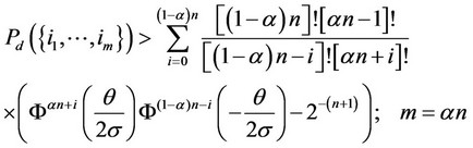 (10)
(10)
Proof Considering q/s asymptotically large, we first approximate  by 1, in Expression (4). We then, use expression (5) and consider again asymptotically large values of q/s. The result proves that the probability in (4) converges to 1, as q/s approaches infinity.
To derive the bound in (9), we first bound
 from below by F(–w) in the integrand of expression (4). Then, we use Equation (7) on the resulting integral expression.
To derive the bound in (10), we bound  from below by: 1) F(q/s); for negative w values and 2) by F(–w); for positive w values. We then use Expressions (5) and (8) from the Corollary.
Lemma 2 below states a probability of correct detection result for the case where the percentage of signalincluding observations and the signal-to-noise ratio are both very small.
Lemma 2 Let a ® 0 and q/s ® 0. Then, the probability of correct detection in (4) is of order an Fn(q/s).
Proof We brake the integral in (4) into two parts: the part from −µ to 0 and the part from 0 to q/2s. For the first part, we expand  via Taylor series expansion to first order q/s approximation. For the second part, we approximate the integral by q/2s times the value of the integrand at zero. Then, we approximate 1 – a » 1. As a result, we then obtain:
 (11)
(11)
We note that, in general, the probability of correct detection induced by the ML optimal detector is of the order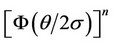 , increasing exponentially to 1; with increasing signal-to-noise ratio q/s, while it is also decreasing exponentially to 0; with increasing sample size.
4. The Outlier Resistant Detector
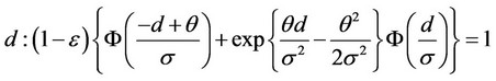
In this section, we consider the case where extreme occasional outliers may be contaminating the Gaussian environment of Section 3. Then, instead of white and Gaussian, the noise environment is modeled as white with pdf belonging to a class F of density functions, defined as follows, for some given value e in (0, 0.5), where ε represents the outlier contamination level:
F = {f;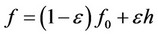 , f0 is the Gaussian zero mean and standard deviation s pdf, h is any pdf}.
The outlier resistant robust detector is then found based on the least favorable density f* in class F above, where the Kullback-Leibler number between f* and its shifted by location parameter q version attains the infimum among the Kullback-Leibler numbers realized by all pdfs in F [6,7]. As found in [7], the log likelihood ratio in (2) is a truncated version of that used in Section 3, As a result, for q > 0, the ML robust detector is operating as follows:
Robustl ML Detector 1) Given the sequence , compute all
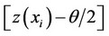 ; 1 £ j £ n, where,
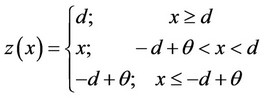 (12)
(12)
 (13)
(13)
2) If ; for all k, 1 £ k £ n, then, decide that no observation contains signal.
3) If $ a set of integers ; 1 £ m £ an:
 ; for all
  and
and
 ; for all, then decide that the observations containing the signal are all those with indices in the set
 .
.
4) If $ a set of integers ; m > an:
 ; for all
  and
and
 ; for all
 , then decide that the observations containing the signal are those whose indices k are contained in the set
  and whose
  values are the αn highest in the set.
We will denote by  the probability of correct detection induced by the robust ML detector, given that the noise is Gaussian containing no outliers and given that the signal occurs at the observation indices
 . Then, we can derive the expressions belowwith some extra caution, assuming again that αn is an integer:
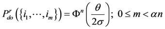
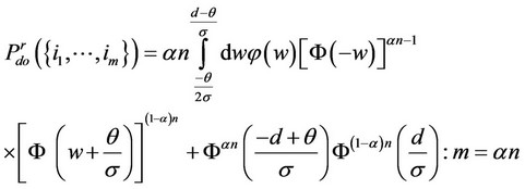 (14)
(14)
Comparing Expressions (4) and (14), we notice that the robust detector induces lower probability of correct detection at the nominal Gaussian model; for the case of m = an, where the difference of the two probabilities decreases monotonically with decreasing contamination level ε. As we will see in the sequel, this loss of performance of the robust detector at the nominal Gaussian model is at the gain of resistance to outliers.
Let there exist a small positive value ς, such that the noise per observation is zero mean Gaussian; with probability 1 − ς, and is an infinite positive value y; with probability ς. We express below the probabilities
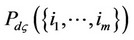 and
and 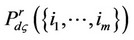 induced by this outlier model and the optimal ML detector in Section 3 versus the robust detector, respectively.
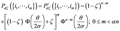 (15)
(15)
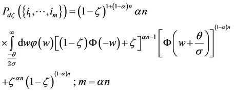 (16)
(16)
 (17)
(17)
Comparison between Expressions (16) and (17) reveals that the robust detector attains higher probability of correct detection than the detector in Section 3; in the presence of the extreme outliers, where the difference of this performance increases with increasing ς value.
Remarks If it is known that the signal may appear as a set of bursty batches of unknown sizes and protection against data outliers is needed, then, the robust re-initialization sequential algorithm in [9] will sequentially detect the beginning and the ending of each batch with minimal complexity, no memory requirements and with accuracy increasing with the signal-to-noise ratio and the size of each batch. Let then  denote the value of the robust algorithm which detects the beginning of a signal batch, upon the processing of the nth datum xn from its beginning. Let
  denote the value of the robust algorithm which detects the ending of the batch, upon processing the nth datum
  from the beginning of its initialization. The whole algorithmic system operates then as follows, where
  and
and  are two positive thresholds pre selected to satisfy power and false alarm trade offs and where z(x) is as in (12):
1) Process the observed sequence  sequentially starting with the algorithm
  whose values are updated as follows:

Stop the first time n, such that  and declare n as the time when the signal batch begins.
Then, switch immediately to the algorithm  whose values are updated as follows, where time zero denotes the time when the algorithm begins and where yn denotes the nth observed datum after the latter beginning:
2) 
Stop the first time n, such that  and declare that the signal batch has ended.
5. Suboptimal Tree—Search Detectors
In this section, we consider the special case where the αn components of the sparse signal are spread relatively evenly across the n members of the observation set. Then, we wish to devise a detector whose objective is to identify the presence of isolated signal—including observations within clusters of signal-absent observations. In this case, we may draw from the information theoretic concepts of noiseless source coding to devise tree-searchtype detectors for sparse signals, as was done for the transmission/probing of bursty signals [3,4]. In particular, referring to the notation and model in Section 2, where f1(.) and f0(.) are the pdfs of signal-including versus signal-absent observations, respectively and where
 , we define a tree-search detector as follows, considering for simplicity in notation that the size of the observation set is a power of 2:
Tree—Search Detector 1) Given the sequence , compute all g(xj); 1 £ j £ N = 2n.
2) Utilize a sequence {βk} of given algorithmic constants as:
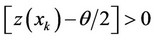
a) If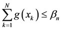 , then, decide that at most a single signal component is contained in the sequence
 .and stop.
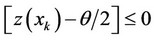
b) If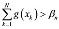 , then, create the two partial sums
  and
and .
.
c) Test each of the two sums in b) against the constant βn–1 and go back to steps a) and b).
3) In general, the observation set  is sequentially subdivided in powers of 2 number of portions, until the subdivision stops. If, during the algorithmic process, the observations with indices
 ; m = 2l are tested, then,
a) If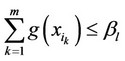 , then, decide that at most a single signal component is contained in the sequence
and stop.
b) If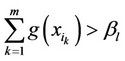 , then, create the two partial sums
  and
and .
.
c) Test each of the two sums in b) against the constant βl–1 and go back to steps a) and b).
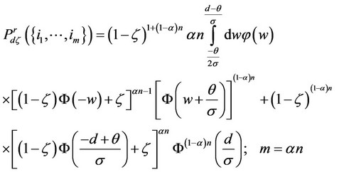
When the signal—including observations are uniformly distributed across all observations, the operational complexity of the tree—search detector is of order [logm] N; where m is the number of signal-including components and N is the size of the observation set. The error performance of the tree—search detector may be studied for general pdfs, asymptotically: that is when the observation set is asymptotically large and each signal—including observation component is isolated in the middle of an asymptotically large population of signal—absent observations. Then, the central limit theorem provides probability of correct detection expressions which are functions of the Kullback—Leibler numbers between the pdfs f1(.) and f0(.). However, in this section, we will focus on the constant signal and additive Gaussian noise model of Section 3, where the function g(x) in the description of the tree—search detector equals x – θ/2. In the latter case, we express the induced probabilities of correct detection in Lemma 3, below.
Lemma 3 Let a constant signal θ be additively embedded in white zero mean Gaussian noise with standard deviation σ. Let m =2l be the number of signal components, given that they are spread uniformly across a total of N = 2n observations, where n > l. Let the constants {βk} used by the tree–search detector be such that: βk < 2βk–1; for all 2 ≤ k ≤ n. Then, the probability, Pd(l, n), of correct detection induced by the tree-search detector is given by the following expression, where this probability is conditioned on the above uniform signal spreading assumption (see Equation (18)).
where,
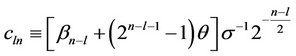 (19)
(19)
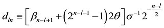 (20)
(20)
Proof For the proof, we consider that a single signal component per 2n–l observations is present. Then, we express Pd (l, n) as the probability that two independent sums of such 2n–l observations are each smaller than βn–l, while their sum is larger than βn–l+1.
It is relatively easy to conclude that the probability of correct decision in (18) is increasing with increasing signal-to-nose ratio θ/σ, as well as with increasing difference n – l. It is also relatively simple to conclude that the βn–l and βn–l+1 values should be of 2–(n–l) order; for asymptotically large values of the difference n – l. We may select the specific values of the constants βn–l and βn–l+1 based on a maximization of correct detection criterion, as stated in Lemma 4 below.
Lemma 4 Let a constant signal θ be additively embedded in white zero mean Gaussian noise with standard deviation σ. Let the signal q occur with probability q per observation, independently across all N = 2n observations. Let Pd (n – l, q) denote then the probability of correctly deciding between at most one and at least two signal components in 2n–l observations, via the use of the tree-search constant βn–l. The constant βn–l may be selected as that which maximizes the probability Pd (n – l, q), where the latter is given by the following expression.
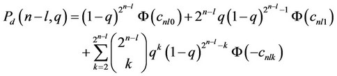 (21)
(21)
where,
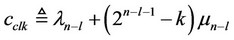 (22)
(22)
 (23)
(23)
 (24)
(24)
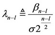
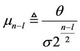
For signal-to-noise ratio q/s asymptotically small, for n – l ³ 2 and , the constant βn–l is given by Equation (25) below, where it can be then shown that βn–l+1 < 2βn–l.

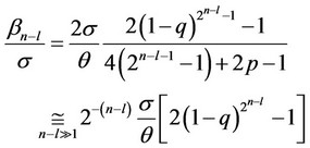 (25)
(25)
Proof Expression (25) is derived in a straight forward fashion. When q/s is asymptotically small, we use first order Taylor expansion approximations with respect to the mn–l (defined in (24)) of the F(.) functions in (21). Subsequently, we find the maximizing ln–l (defined in (23)) value of the resulting expression, as given by (25).
We note that we may “robustify” the tree-search detector at the Gaussian nominal model, by using, instead, g(x) = z(x) – θ/2; for z(x) as in (12). The error performance of the robust tree-search detector may be then studied asymptotically. We will not include such asymptotic study in this paper.
6. Discussion and Conclusion
In this paper, we investigate the problem of detecting sparse signals that are embedded in noise. The effective solution of the problem requires clear modeling of any a priori knowledge available to the designer. We first present and analyze the problem solution when only the highest percentage of signal-including observations is a priori known. In the latter case, we consider the special case of a constant signal embedded in additive white Gaussian noise and presented both parametric and outlier resistant solutions. Secondly, we present an efficient solution to the problem when it is a priori known that the signal occurs in bursty batches. Finally, we present a tree-search solution approach for the case when the sparse signal is known to be uniformly distributed within the observations set. We analyze all our approaches in terms of probability of correct detection performance and complexity.
REFERENCES
- E. J. Candes, J. Romberg and T. Tao, “Robust Uncertainty Principles: Exact Signal Reconstruction from Highly Incomplete Frequency Information,” IEEE Transactions on Information Theory, Vol. 52, No. 2, 2006, pp. 489-509. doi:10.1109/TIT.2005.862083
- J. A. Tropp and A. C. Gilbert, “Signal Recovery from Random Measurements via Orthogonal Matching Pursuit,” IEEE Transactions on Information Theory, Vol. 53, No. 2, 2007, pp. 4655-4666. doi:10.1109/TIT.2007.909108
- J. F. Hayes, “An Adaptive Technique for Local Distribution,” IEEE Transactions on Communications, Vol. 26, No. 8, 1978, pp. 1178-1186. doi:10.1109/TCOM.1978.1094204
- J. I. Capetanakis, “Tree Algorithms for Packet Broadcast Channels,” IEEE Transactions on Information Theory, Vol. 25, No. 5, 1979, pp. 505-515. doi:10.1109/TIT.1979.1056093
- A. T. Burrell and P. Papantoni-Kazakos, “Random Access Algorithms in Packet Networks: A Review of Three Research Decades,” International Journal of Communications Network and System Sciences (IJCNS), Vol. 5, No. 10, 2012, pp. 691-707. doi:10.4236/ijcns.2012.510072
- P. Huber, “A Robust Version of the Probability Ratio Test,” The Annals of Mathematical Statistics, Vol. 36, 1965, pp. 1753-1758. doi:10.1214/aoms/1177699803
- D. Kazakos and P. Papantoni-Kazakos, “Detection and Estimation,” Computer Science Press, 1990.
- A. T. Burrell and P. Papantoni-Kazakos, “Extended Sequential Algorithms for Detecting Changes in Acting Stochastic Processes,” IEEE Transactions on Systems, Man, and Cybernetics, Vol. 28, No. 5, 1998, pp. 703-710. doi:10.1109/3468.709621
- A. T. Burrell and P. Papantoni-Kazakos, “Robust Sequential Algorithms for the Detection of Changes in Data Generating Processes,” Journal of Intelligent and Robotic Systems, Vol. 60, No. 1, 2010, pp. 3-17.