Journal of Signal and Information Processing
Vol.3 No.2(2012), Article ID:19571,8 pages DOI:10.4236/jsip.2012.32029
Direction Finding Using Cumulant in Multipath Environment with an Arbitrary Array
![]()
1Electrical Engineering Department, Islamic Azad University-South Tehran Branch, Tehran, Iran; 2Electrical Engineering Department, Iran University of Science and Technology, Tehran, Iran.
Email: Maryam.Johnny@gmail.com
Received January 3rd, 2012; revised February 8th, 2012; accepted March 13th, 2012
Keywords: Array Interpolation; Direction of Arrival; MUSIC; Cumulant; Uniform Linear Array
ABSTRACT
In this paper, the problem of estimating the direction of arrival of signals of which some may be perfectly correlated is considered. This method can be applied in the situation that the non-Gaussian independent and coherent signals coexist with unknown Gaussian noise. In this method at first via mappings, the virtual uniform linear array (ULA) and also the shifted versions of this virtual ULA by assuming that all the DOAs are located in one section are constructed. In order to avoid coloring the noise because of these mappings we use a cumulant matrix instead of a covariance ones. In this method since we construct all the subarrays virtually for detection of coherent signals we do not need the array with regular configuration. The advantages of this method are: increasing the array aperture, having the ability to find the DOAs with fewer sensors and also avoiding the coupling between sensors as much as possible in contrast to conventional spatial smoothing.
1. Introduction
Direction finding techniques based on the eigendecomposition of the covariance matrix of the vector of the signals received by an array of sensors, have received considerable attention in years. The main drawback of these techniques like MUSIC [1] is their inability to handle perfectly correlated (or highly correlated) signals which arise quite often in practice due to multipath propagation. This fact has motivated various researchers to look for variations of the MUSIC algorithm which do not suffer from this problem. Under the certain conditions, spatial smoothing technique introduced in [2,3] makes it possible to use a MUSIC type algorithm in the presence of arbitrary signal correlation. The most restrictive aspect of the spatial smoothing technique as presented in [2] and discussed further in [3,4], is that it requires a linear uniformly spaced array and also has a significant loss of array aperture. Other techniques, such as the one presented in [5], appear to have similar restrictions. Also these methods all assume that the additive noise is a white Gaussian process or the noise covariance matrix is known in advanced. On the contrary, in many practical situations, the additive noise is colored Gaussian process and a priori estimate of the noise covariance matrix is not available therefore these methods will suffer severe performance degradation. Owing to the attractive property of Gauassian processes that all cumulant spectra of order greater than two are identical to zero, many effective algorithms based on cumulants [6,7] have been proposed. An attempt to generalize the spatial smoothing technique based on cumulant to arbitrary array geometries (Sparse Array) by using the idea of interpolated array [8] is the main topic here. In this method we need no extra sensors and subarrays so array aperture significantly increased means that we need only K + 1 sensors for detection of K coherent signals in contrast to conventional spatial smoothing that needs 2K sensors or FBSS that use  sensors [9]. This paper is organized as follows. A definition of cumulant and some properties of that is introduced in Section 2. Narrowband signal model and also the proposed method of DOA estimation are then considered and analyzed in detail in Sections 3 and 4, respectively. The simulation results to validate the effectiveness of our method are shown in Section 5 and some concluding remarks are given in Section 6.
2. Cumulant for Array Processing
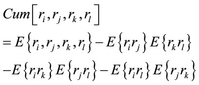
Conventional array processing techniques utilize only the second order statistics of received signals. Second-order statistics are sufficient whenever the signals can be completely characterized by knowledge of the first two moments, as in the Gaussian case; however, in real applications, practical far field sources often emit non-Gaussian signals, e.g., as in a communication scenario. Whenever second-order statistics can not completely characterize all of the statistical properties of underlying signals, it is beneficial to consider information embedded in higher than second-order moments. Higher order prove to be rewarding alternative to second order statistics, and there are many signal processing problems that are not solvable without access to HOS [10]. Particular cases of higher order statistics (Cumulant) are the third and fourth order statistics. In most of the application that deal with cumulant we use fourth order statistic, a logical question to ask is “why do we need fourth order cumulant?” If a random process is symmetrically distributed like Laplace, Uniform, Gaussian, etc. then its third order cumulant equals zero. Additionally, some processes have extremely small third order cumulants and much larger fourth order so for such a process we must use fourth order cumulant. We list properties of cumulants that are useful to us in the sequel [10]:
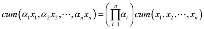
[CP1]—If  are constants and
  are random variables, then
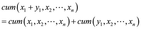
[CP2]—Cumulants are additive in their arguments
[CP3]—If the random variable  are independent of the random variables
  then
then
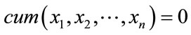
[CP4]—Cumulant suppress Gaussian noise of arbitrary covariance, i.e., if  are Gaussian random variables independent of
  and
and  we have

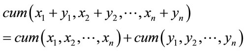
[CP5]—If a subset of random variables  are independent of the rest, then
[CP6]—The permutation of the random variables does not change the value of the cumulant.
In this paper we use Fourth order Cumulant defined as follows:
3. Problem Formulation
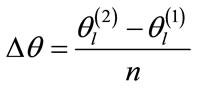
Consider an arbitrary array composed of M sensors. Let q narrowband and non-Gaussian plane waves with zero mean, centered at frequency , impinge on the array with M sensors like Figure 1 from directions
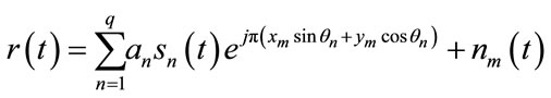
 . Using complex signal representation, the received signals at the mth sensor can be expressed as
 (1)
(1)
where  is the signal associated with the nth wavefront,
  is the complex response of the sensor to the nth wavefront,
 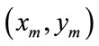 are the coordinates of the mth sensor measured in half wave-length unites and
  is an additive noise at the mth sensor. In addition, the unknown noise is assumed to be Gaussian with variance
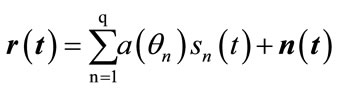
 , uncorrelated with the signals and uncorrelated from sensor to sensor. Rewriting (1) in a vector notation, assuming for simplicity that the sensors are ominidirectional with unit gain, i.e.,
  , we obtain:
 (2)
(2)
where  are the
  vector
 (3a)
(3a)
 (3b)
(3b)
And  is the steering vector of the array in the direction
 :
:
 (4)
(4)
To further simplify the notation, we rewrite (2) as
 (5)
(5)
where S(t) is the  vector as:
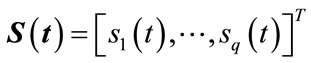 (6)
(6)
and  is the
  matrix
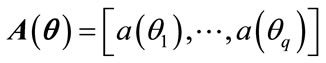 (7)
(7)
also the fourth order cumulant of  can be computed as (8).
 (8)
(8)
For 
The computation of cumulant and some algorithm based on are come in [11]. In this paper for solving noise coloring we use cumulant counterpart instead of a covariance. In fact we replace every member of covariance matrix with its cumulant counterpart which is computed in the sufficient snapshots by (9).
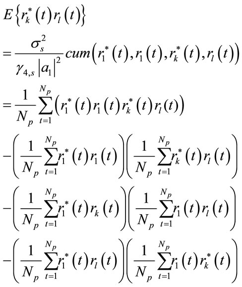 (9).
(9).
4. Proposed DOA Estimation
4.1. Spatial Smoothing
Communication systems operating in a mobile communication environment may encounter multipath propagation caused by various reflected surfaces (e.g., buildings, hills, cars, etc.). When a signal wavefront reflects off of a surface, the original wavefront and the reflected wavefront will both impinge on the receiving array of sensors, although from different directions. Since the original signal and reflected signal come from the same radiating source, if the delay difference between the two paths is sufficiently small, then the signals are coherent (i.e., fully correlated) and their covariance matrix or cumulant matrix is singular. As was pointed out in the previous section, the nonsingularity of the signal covariance matrix or cumulant matrix is the key to successful application of eigenstructure techniques. Many effective decorrelated methods are then proposed to overcome this problem. Among these methods, the spatial smoothing techniques are relatively more effective, which are first introduced in [2] and extensively studied by Shan et al. [3] and Pillai and Kwon [9]. Their solutions are based on a preprocessing scheme that divides the original array into number of subarrays. Then the average of the subarray covariance matrices is computed and in conjunction with the high-resolution methods to resolve the signals. Examination of the smoothing technique described in [13,14] reveals that it is not limited to uniform linear arrays. The forward and also forward-backward spatial smoothing can be performed on any array which can be subdivided into subarrays which all have the same configuration, but are shifted with respect to each other like Figure 2. But when it is urgent to use Sparse array or any array that has not a suitable construction for using spatial smoothing like Figure 1 what should we do for the detection of the K coherent signals?
4.2. Array Interpolation
1) The first step in designing an interpolated array is to divide the field of view of the real arbitrary array into sectors.
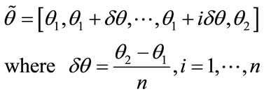
2) For each sector we define a set of angles like 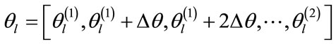 where
where
 . These angles are used only in the design of the interpolation matrix.
3) Compute the steering vectors associated with the set
 for the given real array and arrange them in a matrix as follows:
 (10)
(10)
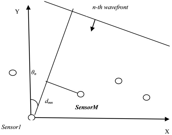
Figure 1. An arbitrary geometry.
Figure 2. Subarray with the same configuration [14].
Next we decide where we want to place the virtual elements of the interpolated array, having decided on their locations we can compute the array manifold of the interpolated array. We denote by  the section of this array manifold computed for the angles
  also as follows:
 (11)
(11)
In other words ,
,  are the responses of the real and virtual arrays to the signals arriving from the set
  respectively. In this paper we try to create virtual subarrays having a suitable geometry for the application of the spatial smoothing technique. The idea in this paper is to select the uniform linear arrays as the virtual subarrays all having the same number of sensors as the originnal real array but are shifted versions of each other like Figure 3. The displacement vector of these virtual subarrays and also between their sensors is equal to
 .
.
4) The basic assumption is that the array manifold of the virtual array can be obtained by linear interpolation of the array manifold of the real array, within each sector. In other words, we assume that there exist a constant  matrix
  such that
 (12a)
(12a)
Of course, the interpolation is not exact and therefore the equality above does not really hold. The “best” interpolation matrix  is the one which will give the best fit between the interpolated response
  and the desired response
 .
.
In this paper we assume that all the coherent DOAs are located in one section like , this section is divided with the calibration angles
 .
.
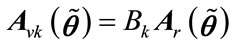
where n is the division index,  are the manifold matrixes for the kth desired virtual subarray and real array respectively constructed from these calibration
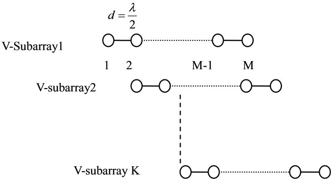
Figure 3. Virtual subarrays.
angles . Because every virtual subarray is the shifted version of the first virtual subarray. So:
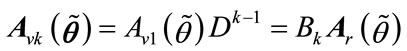 (12b)
(12b)
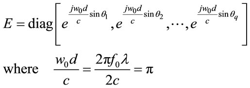
where  denotes the kth power of the
  diagnal matrix D as follows:
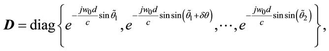
 (13)
(13)
In (13) parameter c is the speed of light and d is the distance between adjacent sensors of virtual ULA that for avoiding grating lobe it must be equal to half a wavelength . By the idea of interpolation as described in 4.2 we can relate every virtual subarray to the real ones by solving a following linear equation:
 (14)
(14)
In following we use the cumulant’s properties in the direction finding. Since the Cumulant or Fourth order moment is blind to additive Gaussian noise (color or white) as shown in (CP4) the Fourth order Cumulant matrix counterpart of the real array is obtained as follows:
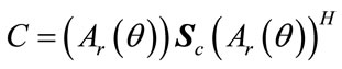 (15a)
(15a)
where  is the
  Cumulant matrix of signals that impinge on the real array. After obtaining interpolation matrix
  for every virtual subarray now we can compute the cumulant of these subarrays as follows:
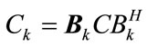 (15b)
(15b)
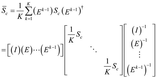
Now the spatially smoothed cumulant matrix is defined as the sample means of the virtual subarrays cumulants:
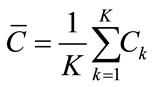 (16)
(16)
where K is the number of virtual subarrays that for nonsingularity of  it should be larger than the number of coherent signals. If mapping matrices
  best selected then
  becomes:
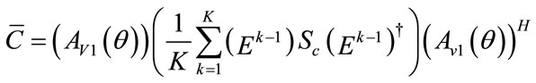 (17)
(17)
And  is the kth power of E.
From (17) we can define  as follows:
 (18)
(18)
Which can be further simplified to:
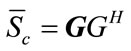 (19)
(19)
where  is the
  block matrix:
 (20)
(20)
In which  denoting the Hermitian square root of
 . It is clear that the rank of
  is equal to the rank of
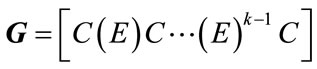
 . Thus our task is to prove that G has rank q even when this q signals are coherent. Recalling that the rank of a matrix is unchanged by a permutation of its columns, it can be easily verified that G can be written in the form of (21).
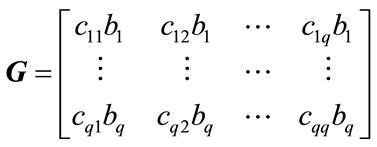 (21)
(21)
where  is the ijth element of the matrix
  and
and  is the
  column vector:
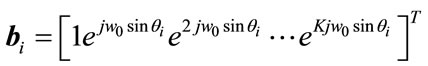 (22)
(22)
To show that the matrix  is of rank q, it suffices to show that each row of the matrix S has at least one nonzero element and that all the vectors
  are linearly independent. The first fact follows by contradiction. Assume that a row of
 , say the kth, is composed of all zeros this implies that the kth signal has zero cumulant, in contradiction to the definition of
  as the cumulant matrix of nonvanishing non-Gaussian signals. The linear independence of the vectors
  follows by observing that these vectors can be embedded in a vandermonde matrix. Since rank of
  is equal to the rank of
  and rank of
  is
is  so the rank of
  is
is . At the end we apply one of the subspace methods to
 .
.
5. Simulation and Experimental Results
In this section, we illustrate the performance of our method through simulations. We select conventional spatial smoothing in the presence of white noise with variance  as a comparative method. In the first simulation, we consider three non-Gaussian coherent signals received by two arrays, ULA for the Conventional Spatial Smoothing and the known arbitrary one for our Cumlant Spatial Smoothing each with 7 sensors. The amplitudes and phases of the complex fading coefficient of coherent signals are
  and
and 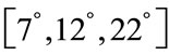 respectively. The unknown colored Gaussian additive noises are generated by passing the complex white Gaussian random processes with zero mean and
  variance through a spatial moving average (MA) filter of order 2 with coefficients
 , where
  are selected to be
  in the simulations. The input SNR is defined as
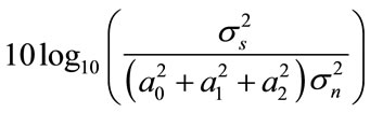 . Note that the noise covariance matrices for colored and white noises have the same trace, i.e. total noise power introduced to these methods have the same power. 200 Monte Carlo trials were performed for each experiment, and the root mean square error (RMSE) of the DOA estimates is used as the performance index:
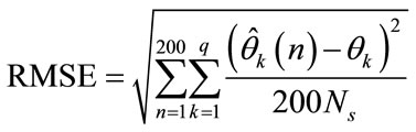
where  is an estimate of
  for the nth Monte Carlo trial, and
  is the number of all the independent or coherent signals. In Figure 4 the RMSE of the DOA estimates against input SNR is shown with the Ns = 500 and 1000 snapshots for the two methods. Also the RMSE of the DOA estimate of two methods versus the number of snapshots with input SNR equaling to zero is shown in Figure 5. In these two simulations we assume that the division index is n = 50 for our method. As it is clearly seen, the performance of our method (Cumulant Spatial Smoothing) is better than Conventional spatial smoothing

Figure 4. RMSE of the DOA estimates against input SNR for coherent signal.

Figure 5. RMSE of the DOA estimates against number of snapshot.
specially in low SNR but against the increasing of snapshots. In the third simulation we show the performance of our method versus division index n in the presence of three predefined coherent signals. As it is obvious in Figures 6(a)-(c), by choosing n as large as possible we can get a better resolution (targets are distinguished clearly). To investigate the performance of our cumulant based method, we performed additional experiments by changing both the SNR and the data length. Each mean and standard deviation pair in each table are obtained from 100 independent realizations. Table 1(a) reports the results of Spatial Smoothing for 200 snapshots with different SNRs in which the conventional spatial smoothing based on sample covariance means is selected as a direction finder method. Table 1(b) also shows the performance of conventional spatial smoothing versus two different snapshots with SNR equaling to zero.
From Tables 1(a), (b) it is obvious that the conventional spatial smoothing is more dependent on SNR than snapshot and can estimate DOAs with fewer snapshots by increasing the SNR accurately. Also we repeat the experiment again for our method based on the sample cumulant means with division index n = 50, as it is seen in Table 2(a) we can obtain better estimations in the low SNR by increasing the number of snapshots or data lengths. Table 2(b) also shows the performance of our method versus two different SNRs with a number of snapshots equaling to 200.
As shown in Table 2(b) our cumulant spatial smoothing fails in general in a few snapshots, it means that the effect of snapshots in our method is more than the SNR in contrast to conventional spatial smoothing. In the latter simulation we do the detection probability for these two
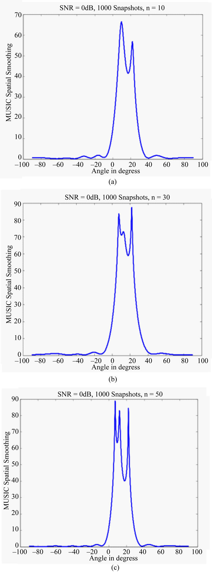
Figure 6. (a)-(c) Effect of division index (n) for a narrow sector on the resolution of our cumulant spatial smoothing.
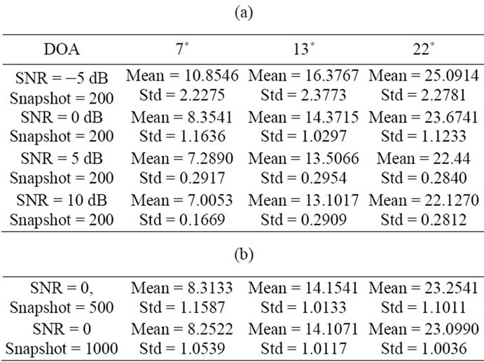
Table 1. (a) (b), DOA estimation with conventional spatial smoothing with 7 sensor versus SNR and snapshot.
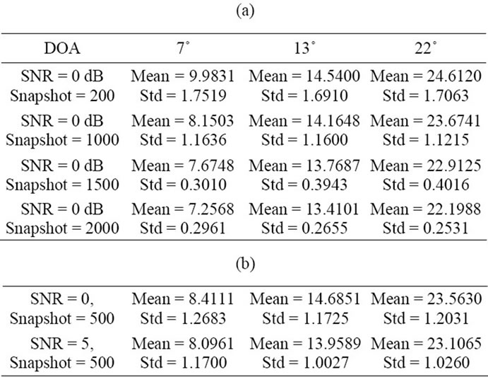
Table 2. (a) (b), DOA estimation with our cumulant method with 7 sensors versus SNR and snapshots.
methods (Cumulant and conventional spatial smoothing). This detection is computed over 250 independent trails by detecting the source(s) at  within an interval of
  around this actual DOA. Figure 7 shows this detection probability for our cumulant spatial smoothing with three different ns and also conventional spatial smoothing versus SNR. As it is clearly seen by increasing the n we can get better detection probability. As the explanation of Figure 7 we must say that the detection probability of our method is more depend on mapping matrix
  obtained from solving Equation (14). We see that by selecting n as large as possible we can obtain the best mapping matrix as in [15-17] has been said.
6. Conclusion
In this paper, DOA estimation method in multipath environment with fewer sensors has been presented. We have taken the effects of cumulant and interpolated array into
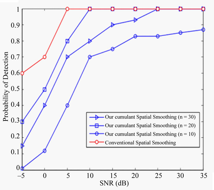
Figure 7. Probability of detection versus SNR and n.
account in spatial smoothing. In this paper, by the use of mapping and interpolation techniques in an arbitrary array geometry we tried to approach to the ULA and also shifted versions of this ULA so that the spatial smoothing can be performed on it, therefore the need for extra real subarrays has been removed. Because this mapping can color the white noise and also in practical situation we don’t have any knowledge of Gaussian noise, we use cumulant instead of the covariance of data. The simulation results presented illustration of the performance of our method against n, SNR and the number of snapshots. We see by increasing these parameter the resolution and the probability of detection of our method will be better.
REFERENCES
- A. J. Barabell, “Improving the Resolution Performance of Eigenstructure Based Direction Finding Algorithms,” Proceedings of the International Conference on Acoustics, Speech, and Signal Processing, Boston, Vol. 8, 1983, pp. 336-339.
- T. J. Shan and T. Kailath, “Adaptive Beamforming for Coherent Signals and Interference,” IEEE Transactions on Acoustic Speech and Signal Processing, Vol. 33, No. 3, 1985, pp. 527-536. doi:10.1109/TASSP.1985.1164583
- T. J. Shan, M. Wax and T. Kailath, “On Spatial Smoothing of Estimation of Coherent Signals,” IEEE Transactions on Acoustics, Speech and Signal Processing, Vol. 33, No. 3, 1985, pp. 806-811. doi:10.1109/TASSP.1985.1164649
- S. U. Pillai and B. H. Kwon, “Performance Analysis of MUSIC-Type High Resolution Estimators for Direction Finding in Correlated and Coherent Scenes,” IEEE Transactions on Acoustics, Speech and Signal Processing, Vol. 37, No. 8, 1989, pp. 1176-1189. doi:10.1109/29.31266
- J. A. Cadzow, Y. S. Kim and D. C. Shive, “General Direction of Arrival Estimation: A Signal Subspace Approach,” IEEE Transactions on Aerospace and Electronic Systems, Vol. 25, No. 1, 1989, pp. 31-47. doi:10.1109/7.18659
- M. C. Dogan and J. M. Mendel, “Application of Cumulants to Array Processing—Part I: Aperture Extension and Array Calibration,” IEEE Transactions on Signal Processing, Vol. 43, No. 5, 1995, pp. 1200-1216. doi:10.1109/78.382404
- S. Lie, A. R. Leyman and Y. H. Chew, “Fourth-Order and Weighted Mixed Order Direction-of-Arrival Estimators,” IEEE Signal Processing Letters, Vol. 13, No. 11, 2006, pp. 691-694. doi:10.1109/LSP.2006.879456
- M. Johnny, M. Johnny and V. T. Vakili, “Wideband Direction Finding Using Cumulant in Arbitrary Array,” IEEE International Conference on Acoustic, Speech, and Signal Processing, Victoria, October 2011, pp. 135-139.
- S. U. Pillai and B. H. Kwon, “Forward/Backward Spatial Smoothing Techniques for Coherent Signal Identification,” IEEE Transactions on Acoustics, Speech, and Signal Processing, Vol. 37, No. 1, 1989, pp. 8-15. doi:10.1109/29.17496
- M. C. Dogan and J. M. Mendel, “Applications of Cumulants to Array Processing—Part I: Aperture Extension and Array Calibration,” IEEE Transaction on Signal Processing, Vol. 43, No. 5, 1995, pp. 1200-1216.
- P. Chevalier, A. Ferreol and L. Albera, “ High Resolution Direction Finding from Higher Order Statistics: The 2qMUSIC Algorithm,” IEEE Transactions on Signal Processing, Vol. 55, No. 11, 2008, pp. 5337-5350. doi:10.1109/TSP.2007.899367
- R. O. Schmid, “Multiple Emitter Location and Signal Parameter Estimation,” IEEE Transactions on Antennas and Propagation, Vol. 34, No. 3, 1989, pp. 276-380. doi:10.1109/TAP.1986.1143830
- M. J. D. Rendas and J. M. F. Moura, “Resolving Narrowband Coherent Paths with Nonuniform Arrays,” Processing of the International Conference on Acoustics, Speech, and Signal Processing, Glasgow, 1989, pp. 2625-2628.
- H. Y. Wang and K. J. R. Liu, “2-D Spatial Smoothing for Multipath Coherent Signal Separation,” IEEE Transactions on Aerospace and Electronic Systems, Vol. 34, No. 2, 1999, pp. 391-405. doi:10.1109/7.670322
- P. Hyberg, J. Magnus and B. Ottersten, “Array Interpolation and DOA MSE Reduction,” IEEE Transactions on Signal Processing, Vol. 53, No. 12, 2005, pp. 4464-4471. doi:10.1109/TSP.2005.859341
- G. H. Glob and C. F. Van Loan, “Matrix Computation,” Johnn Hapkins University Press, Baltimore, 2007, pp. 425- 426.
- M. Johnny and M. Johnny, “Wideband Radar with Detecting and Tracing Corona Arc around Any High Speed and Anti-Radar Aircraft,” Proceedings of Cambridge-Progress in Electromagnetic Research Symposium, Boston, 2010, pp. 75-80.