American Journal of Plant Sciences
Vol.3 No.10(2012), Article ID:24143,4 pages DOI:10.4236/ajps.2012.310173
Bioclimate-Vegetation Interrelations along the Pacific Rim of North America
![]()
1Instituto Universitario de Investigación en Estudios Norteamericanos “Benjamin Franklin”, Universidad de Alcalá, Alcalá de Henares, Spain; 2Facultad de Ciencias, Universidad Autónoma de Baja California, Ensenada, Mexico; 3Departamento de Estadística e Investigación Operativa, Universidad de Granada, Granada, Spain; 4Departamento de Ciencias Ambientales, Universidad de Guadalajara, Guadalajara, Mexico.
Email: *peinado.manuel@gmail.com
Received July 20th, 2012; revised August 20th, 2012; accepted August 31st, 2012
Keywords: Bioclimatology; Boreal Forests; Mediterranean Vegetation; Plant Formations; Temperate Rainforests; Zonobiomes
ABSTRACT
This study was designed to examine relationships between climate and vegetation of the Pacific rim of North America, from the Mediterranean deserts of California to Alaska’s boreal taiga. Relations were inferred from temperature and rainfall data recorded at 457 weather stations and by sampling the vegetation around these stations. Climate data were used to construct climatograms, calculate forty one variables and detect main latitudinal and longitudinal gradients. In order to identify the best functions able to relate our variables, polynomial and non-polynomial regressions were performed. The k-means algorithm was the clustering method used to validate the variables that could best support our bioclimatic classification. The variable that best fitted our classification was finally used to prepare a discriminatory key for bioclimates. Across this extensive area three macrobioclimates were identified, Mediterranean, Temperate and Boreal, within which we were able to distinguish nine bioclimates. Finally, we relate the different types of potential natural vegetation to each of these bioclimates and describe their floristic composition and physiognomy.
1. Introduction
Vegetation science, like any other science, uses classification to understand the laws of Nature, and organize knowledge. Bioclimatic classification schemes attempt to relate meteorological data to the geographic distribution areas of living organisms, mainly of single plant species or plant communities. World zones showing marked climatic gradients can be the best laboratory to assess whether the vegetation’s distribution follows a climatic pattern, as reflected by meteorological data.
The Pacific coast of North America with a general climate that is driven by oceanic currents (the Humboldt Current in the south, the Aleutian-California current in the north) is an area of particular bioclimatic interest owing to its drastic north-south gradient embracing tundras, coastal rainforests, temperate and Mediterranean forests, Mediterranean scrubs, and deserts. Although this is well-known and mentioned in practically every general geobotanical survey (for references see [1,2]), we still lack a detailed description of the bioclimatic patterns and transitions that occur along this dramatic gradient and its impacts on the distribution of vegetation types.
Several published reports exist on the bioclimatology of North America [3-6]. These surveys have been based on the classification into zonobiomes of Walter [7] and on the successive bioclimatic schemes proposed by RivasMartínez, which have led to a worldwide bioclimatic classification system [8]. Several authors have also described the vegetation of the area examined here, but so far no investigation within a given study area has tried to relate the types of vegetation identified in field work to climate data provided by the meteorological stations of the selected area.
Following Walter’s and Rivas-Martinez’s concepts, but using real field data, the main objective of the present study was to identify the climate variables that would best discriminate existing bioclimates and potential natural vegetation along the Pacific rim of North America between the Mexico-United States border in California and Alaska. A bioclimate was here defined as an eclectic biophysical model described by means of climate variables and vegetation types [4], mainly those regarded as potential natural vegetation (PNV), i.e., the climatophilous plant community that would become established if all successional sequences were completed without human interference under the present climate and edaphic conditions [9]. As support for this bioclimatic interpretation, two statistical methods—regression analysis and cluster analysis—were used to determine the lowest possible number of simple climate factors that could define and predict the vegetation distribution changes observed.
2. Materials and Methods
2.1. Study Area
Overlooking the Pacific Ocean, the study area covers an airline distance of approximately 4100 km from Cook Inlet, AK (the northernmost weather station examined was Skwentna, at 61˚58'N) to southern CA (where the southernmost station was Campo, at 32˚37'N). Its western limit is Port Heiden, AK, at 158˚37'W, while the easternmost site examined was 116˚25'W, in Borrego Desert, CA. The whole area forms part of the largest and highest of North American physiographic systems, the Pacific Border System [1], which is the backdrop for most of the ocean’s shores. Two parallel belts of mountains dominate the area. In the north, the Alaska, Chugach and Saint Elias ranges of AK and British Colombia (BC), the BC Coastal Ranges and the Insular Mountains of the islands of Queen Charlotte and Vancouver, constitute a seaward fringe of peaks. To the south, the Coast Ranges between northern CA, Oregon (OR) and Washington (WA) (including the Olympics) dominate the outer coastal topography. These coastal mountains act as effective barriers to the moisture-laden westerly winds, and rainshadow plateaus, depressions and valleys form downwind (Figure S1 as supplementary material at http://foto.difo.uah.es/geobotanica/ficheros/peinado). From the Fraser River Valley, in southeast BC, southwards, across WA and OR, the piedmonts of the Cascades define the eastern boundary.
According to the macrobioclimate (MB) classification system used in our previous studies for western North American zonobiomes, the study area shows three broad MBs: Boreal, Temperate and Mediterranean [3]. The central zone of the Pacific coast, between OR and BC, shows a Temperate MB, characterized by mild wet winters, cool relatively dry summers, and a long frost-free season. In the northwestern corner of BC and especially along the coast of southeastern AK, the winters are colder and a very oceanic variant of the Boreal MB prevails. Zones of highly continental Boreal MB occur in the lee of the Coastal Ranges in northwestern BC and interior AK. The interior climate is very continental: summers are short but relatively warm; winters are long, extremely cold, and dry. Also, although precipitation is light, evaporation is minimal and permafrost impedes drainage, so bogs and wetlands are common [10].
During all seasons, the prevailing westerly winds in the study area are moisture-laden due to their journey over relatively warm seas. In winter, the land is colder than the ocean, and precipitations along coastal lowlands are frequent. In the southern part of the study area, the land along the coast is warmer than the ocean during the summer and, consequently, when the wind reaches the low coastal area there is little or no precipitation and the Mediterranean MB dominates.
Dice [11] included the boreal and temperate climate zones within the Hudsonian (continental boreal), Sitkan and Aleutian (oceanic boreal) and Oregonian (temperate) biotic provinces. The winter rain zone corresponds to the Californian Region, whose provinces, Northern California and Southern California, are included in the study area. For a more detailed phytogeographical classification, see [12,13].
2.2. Climate and Vegetation
Before conducting fieldwork, a geographic information system (GIS) was designed using ArcMap 9.3 software and the digital terrain model (DTM) of the University of California, Davis (http://www.diva-gis.org/Data). Into this GIS, we entered all the available weather stations providing climatological normals [14] for the study area. To avoid large deviations due to continentality and altitude effects, an essential criterion in the final selection process was that every station had to be less than 100 km away from the sea and 1000 m below sea level. Four hundred and fifty-seven weather stations fulfilled these requirements (Figure 1), and climate data for each station were compiled from [15] for the US stations, and [16] for the Canadian ones.
Next, by combining DTM and satellite images (http://earth.google.com) three variables were calculated for each station: 1) Distance to the shoreline in a straight line always in a westerly direction; 2) Orientation with respect to prevailing moisture-laden westerlies; and 3) Orographic position. Accordingly, the stations were then grouped into three categories (Figure 2): COAST, grouping stations on coastal plains, approximately at sea level, directly accessed by wet fronts. One hundred and sixtytwo stations included in this category show the highest rainfall records (average P: 2088 mm); WIND, describing stations on the windward slopes of the Coastal Ranges and Cascades. Rainfall in these 60 stations is lower than in the previous group (average P: 1495 mm), but in areas with less rain (Figure 2: Mediterranean and Submediterranean) this type or orographic rainfall prevails; and LEE, stations influenced by the rainshadow. Rainfall records in those 235 stations are significantly lower (average P: 946
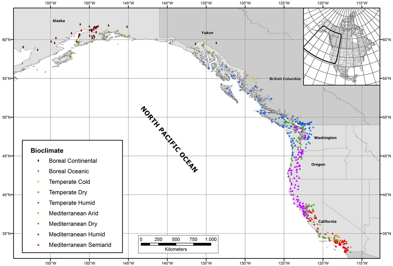
Figure 1. Locations of the weather stations sampled. More detailed maps and geographical coordinates are provided in electronic supplementary material (Maps S1 to S4 and Table S1, respectively).
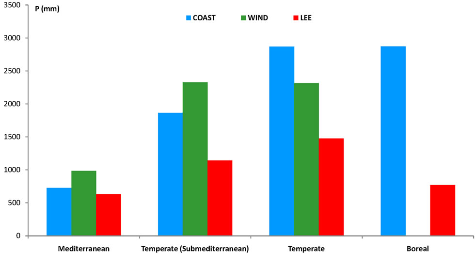
Figure 2. Distribution of average precipitation for three categories of stations, which were in turn grouped into four climate groups, as discussed in the results section. COAST: 162 stations located on coastal plains, approximately at sea level, directly accessed by wet fronts. Stations included in this category show the highest rainfall records (average precipitation: 2088 mm). WIND: 60 stations found on the windward slopes of the Coastal Ranges and Cascades. Rainfall in these stations is lower than in the previous group (average precipitation: 1495 mm), but in areas with less rain (Mediterranean and Temperate Submediterranean) this type or orographic rainfall prevails. LEE: 235 stations influenced by the rainshadow. Rainfall records are significantly lower (average precipitation: 946 mm). Note the prevalence of windward rains in the two areas showing lower precipitation.
mm). Four maps showing DTM and station categories are available as supplementary material (Maps S1 to S4).
Using climate data from weather stations, several parameters and indices were calculated (Table 1). Besides the indices calculated by us, we also used some of those included in the classification schemes of Holdridge [17], Rivas-Martínez [8], Thornthwaite’s index calculated by the method of Dingman [18], and the climatograms of Walter and Lieth [7] which were constructed using the program BIOCLIMA (Alcaraz pers. comm.). Climate data,
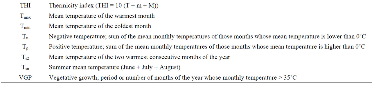
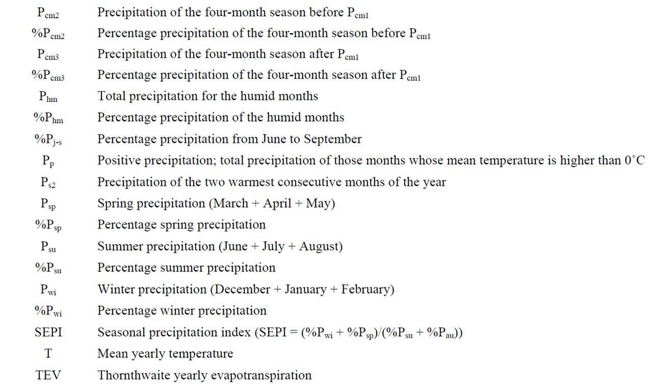
Table 1. Climate data, parameters and indices.
variables and indices for each station are available as electronic supplementary material (Table S1).
Each weather station was initially assigned to a particular PNV using both bibliographical sources and our field data acquired since 1989. In subsequent fieldwork, this classification into vegetation types was checked for 440 of the weather stations. Fieldwork was conducted at sites near each station selected by examining satellite images (http://earth.google.com) to ensure the presence of natural vegetation that was relatively well preserved. These sites were visited from 2003 to 2011. At each site, we first subjectively selected a stand according to the homogeneity of its physical features, vegetation structure and species dominance. The environmental data collected for each stand were elevation, slope, aspect, type of soil, and geological substrate.
Data on vegetation were obtained by plotless sampling, taking censuses of vascular plants at each stand. We recorded the dominant species and their corresponding ecophysiognomic characters, following the basic life forms of Raunkiaer adapted by Ellenberg and Mueller-Dombois [19]. According to the dominant species and vegetation structure, each station was definitively assigned to one PNV. For the 17 stations that could not be sampled in the field, the PNV was inferred using bibliographical sources, satellite images, aerial photograms and by comparing their weather data to those of the stations visited Plant nomenclature follows [20].
2.3. Statistical Analysis
Climate data, parameters and indices in Table 1 were used as variables in the statistical tests: Regression Analysis and Cluster Analysis (CLA). The former emphasizes gradients of continuous variation while the latter produces discontinuous groups.
In order to identify the best regression function able to relate our variables, polynomial and non-polynomial regressions were performed. Regression analysis is a common statistical technique to express, through a mathematical function, the relationship between the independent variable x (climate variables in our study) and the dependent variable y (latitude and longitude in our study). These regression types have been used to describe phenomena in many scientific fields [21]. The adjusted R-squared coefficient (R2) was the criterion used to select the best regression in each case. The higher the value of this coefficient, the stronger the relationship between the variables considered. In most of our analysis, the best regression detected was using polynomial functions. In a limited number of cases no polynomial functions to relate variables appeared. Polynomial and no polynomial functions, together with their respective R2, are represented in Tables 2 and 3.
Since statistical analysis should be conducted when employing heuristics to estimate the probability of incurrect outcomes [22], through CLA we checked the indices and algorithms heuristically obtained by us in previous non-statistical analyses. Among the different CLA techniques, the k-means algorithm is a partitioned, non-hierarchical data clustering method suitable for classifying large amounts of data into a given number . It is the simplest and most commonly used algorithm that employs a squared error criterion. Provided with a set of n numeric objects (number of stations in our case) and an integer number k (BIOs or MBs in our case), it calculates a partition of patterns in k clusters [23]. Once we had defined the groups identified as BIOs through prior climate analyses and fieldwork, the goal of CLA was to identify the climate variable or set of climate variables that could best distinguish some groups from others and to confirm our hypothesis of separation into BIOs. The variable that best fitted our hypothesis was finally used to prepare a discriminatory key for MBs and BIOs.
3. Results
Despite the influence of local factors such as altitude, aspect and orography on the rainfall and temperature data recorded for each sampled station, our results reveal several latitudinal and longitudinal gradients in the study area (Tables 2 and 3).
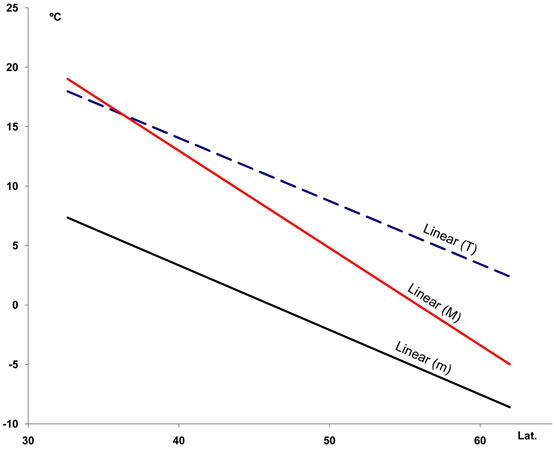
1) Two temperature gradients exist whereby T, M, m, Tsu, Ts2 and Tp decrease with increasing latitude and decreasing longitude, whereas Tn increases approximately north of 58˚ (Figures 3(a) and (b); for abbreviations of climate variables see Table 1).
2) The most significant trend in rainfall detected was its seasonal pattern. Hence, %Psu, %Pau and %Pcm1 in- crease as latitude increases, whereas %Pwi and %Psp rains decrease (Figure 3(c)). These seasonal changes are also reflected in the increasing latitudinal and longitudenal gradients observed in OTI2w, OTI2, OTI3 and OTI4 (Figure 3(d)). Most dramatic effects were detected for the interior boreal stations of Alaska, which showed a seasonal rhythm whereby summer or autumn were the rainiest (Pau > Psu > Pwi > Psp or Psu > Pau > Pwi > Psp) contrasting with the rest of the study area, in which winter is always the rainiest season and summer the driest (Figure 4).
3) Although there is a clear increase in precipitation with latitude (P ranges from 135.6 mm in Pearblossom, California, to 5.728 mm in Little Port Walter, Alaska), the general gradient of increasing rainfall is masked by the rainshadow effect in the lee of the coastal mountains (Figure 5).
Precipitation and temperature gradients cause a similar bioclimatic gradient (Figure 6) reflected by different types
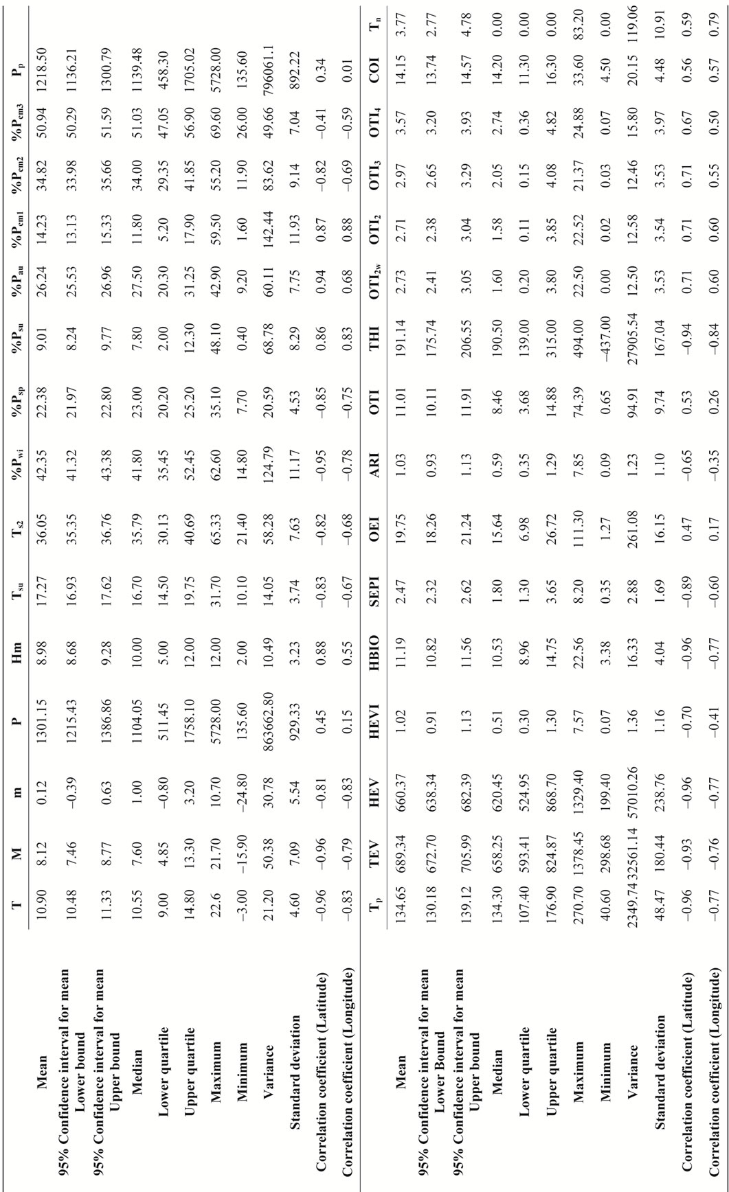
Table 2. Climate data, parameters and indices: summary of the main statisticals values. All correlations are significant at the 0.01 level. For abbreviations of climate variables see Table 1.
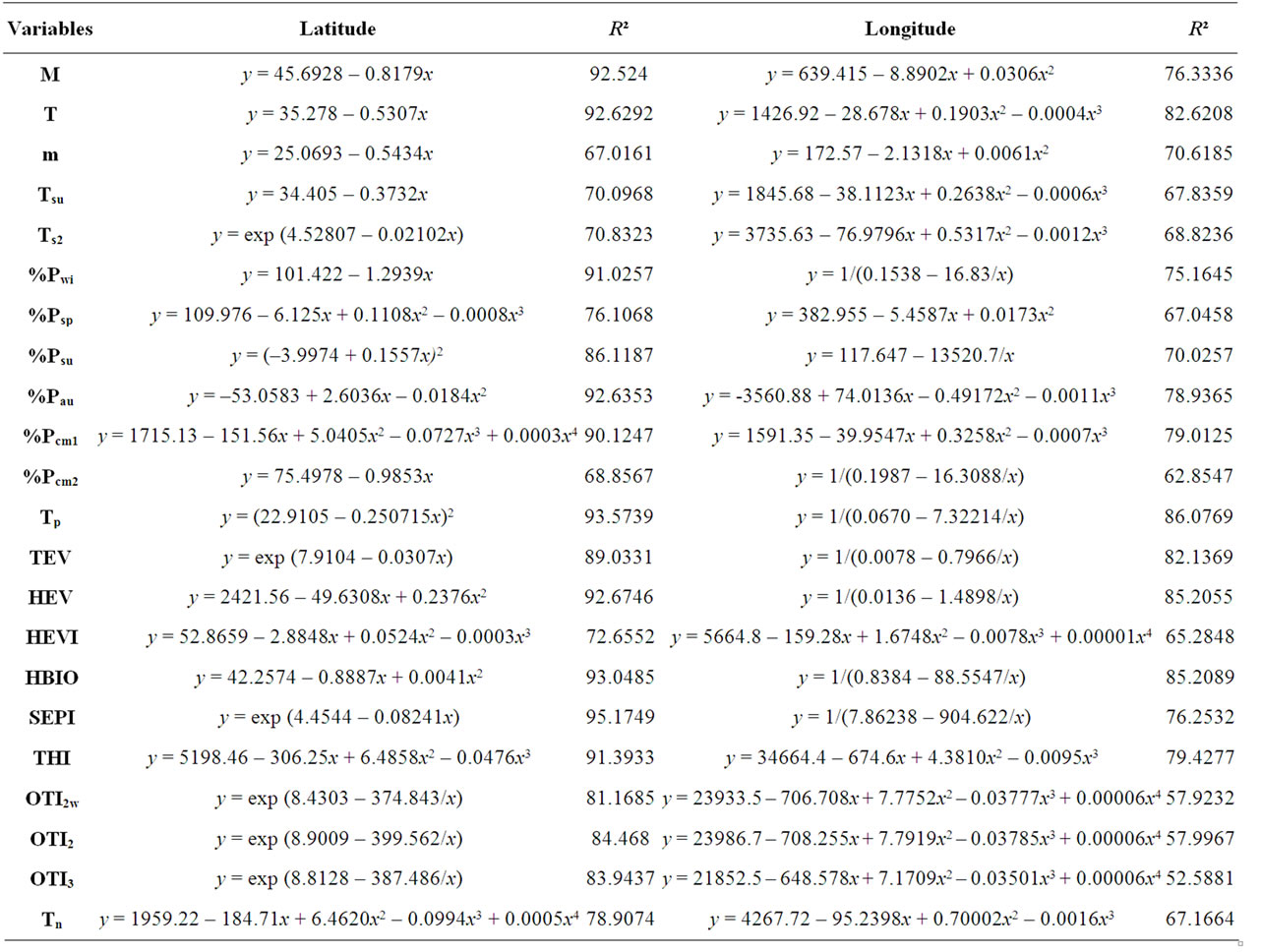
Table 3. Regression fit equations and adjusted R². All the regression functions are significant at the 0.05 level. For abbreviations of the variables see Table 1.
of PNV (Figure 7). Main features of the PNV types are summarized in Table 4. A dichotomous key to PNV based on climate variables is provided as Table 5, and other key based on floristic, phytogeographical, and ecological features as Table 6.
According to CLA, the nine bioclimates discerned in the study area can be distinguished by seven variables (Table 7) that are statistically reliable (Table 8). In Table 8, stations described as “correctly classified” are those found to group together in the CLA with those expected according to our prior hypothesis of belonging to a given MB or bioclimate. It can be observed that even within a high percentage of correct classifications most deviations between real results and CLA results occur in two cases: 1) In the case of MB, when trying to numerically distinguish between Temperate Dry (Submediterranean) and Mediterranean-Humid (CLA 1 and 3) stations. Of less importance is the mismatch in CLA 2, due to 9 temperate and boreal stations of the bordering oceanic zone between British Columbia and Alaska; 2) In the case of bioclimate, when trying to differentiate in frontier zones between Dry and Humid bioclimates (CLA 5 and 6).
4. Discussion
Seasonal patterns of rainfall support the zonobiomes defined by Walter [7] for the study area: ZB IV (Mediterranean), ZB V (Warm-Temperate), and VIII (Boreal). Within this last ZB, Walter distinguishes two climate areas or subzonobiomes: Boreal Cold-Oceanic and Boreal Cold-Continental. Besides, Walter’s classification includes two zonoecotones ZE V-VIII and ZE IV-V. Zonobiomes clearly correspond to the three MBs, Mediterranean, Temperate and Boreal, detected in the study area and, as discussed below, subzonobiomes and zonoecotones can be related to some of the bioclimates described in this article.
By definition, the Mediterranean MB, whose climatic PNV consists mainly of sclerophyllous woody plants, is characterized by, at least, two consecutive dry months during the warmest period in the year; a month is defined as dry if its precipitation is less than twice the temperature
 (a)
(a)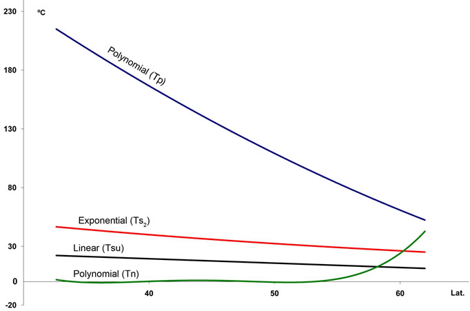 (b)
(b)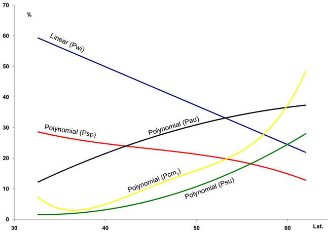 (c)
(c)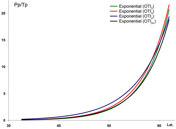 (d)
(d)
Figure 3. Regression lines for seven temperature variables ((a) and (b)), seasonal precipitation percentages (c), and four indices (d) recorded at 457 stations along a north-south transect in the study area. For abbreviations see Table 1. Lat.: Latitude (degrees). For polynomial fit equations and R2 statistics see Tables 2 and 3.
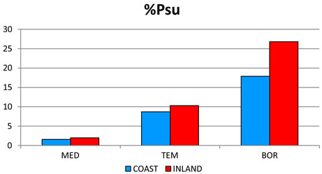
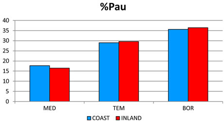
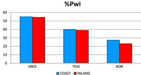
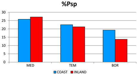
Figure 4. Seasonal precipitation patterns. Percentages for 457 stations distributed according to their position with respect to the wet fronts. For abbreviations see Table 1. The term INLAND included WIND and LEE stations (see Figure 2). MED: 212 stations with a Mediterranean MB; TEM: 184 stations with a Temperate MB. BOR: 61 boreal stations with a Boreal MB.
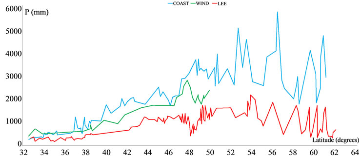
Figure 5. Latitudinal distribution of precipitation for the three categories of stations (see Figure 2). Graphs represent a single value (average precipitation) for all stations in the range of one degree of latitude.
(P < 2T) both measured in mm and ˚C, respectively [7]. The Mediterranean zone of North America spreads from the south of Oregon along the entire California coast until the northwestern corner of Baja California [3]. Inland, the winter-rain region extends northward to British Columbia through the interior valleys of Oregon, Washington and the Puget Sound, always in the lee of the coastal mountains. There, rainfall is so high and summer drought so brief that the forests can be regarded as ZE IV/V [7, p. 166]. Hence, the first step in our statistical analysis was to find an algorithm capable of discriminating Mediterranean and Temperate MBs.
In Mediterranean-Temperate zonoecotones we used a double criterion to consider a station as Mediterranean: 1) Climatically, it should show at least two consecutive drywarm months; and 2) The PNV should be dominated or co-dominated by evergreen trees or shrubs along with some conifers and lateor drought deciduous hardwoods, which are regarded as the typical sclerophyllous vegetation of Mediterranean California, whereas it should lack typical temperate species such as Abies grandis, A. amabilis, Picea sitchensis, Thuja plicata or Tsuga heterophylla.
Of the initial 457 weather stations, 252 show at least two consecutive dry-warm months. One hundred and fifty-seven of these are in California, considered the typical Mediterranean, sclerophyllous region of western North America. All those Californian stations fulfilled these conditions. The other 95 stations that show two dry months outside California share two main features: 1) Arbutus menziesii, Pseudotsuga menziesii var. menziesii (hereafter P. menziesii) and Quercus garryana are always the dominant trees; and 2) They lie in the lee of the Coastal and Vancouver ranges, i.e., rainshadow zones with warm, dry summers and mild, wet winters. In British Columbia, such areas are characterized by the presence of A. menziesii and Q. garryana, whose distribution areas correspond to that of a “modified Mediterranean climate” [24]. In Oregon and Washington, the Arbutus menziesii-Quercus garryana landscape corresponds to the drier climate of the Willamette Valley, Puget Trough and interior valleys of Southwestern Oregon, in the lee of the Coastal Ranges [25,26].
Around these 95 stations outside CA, the PNV can be divided into two groups. In the first group, whose physiognomy is that of a savannah or a woodland dominated by A. menziesii, P. menziesii and Q. garryana, sclerophyllous species are common under the forest canopy, and temperate trees such as Picea sitchensis, Thuja plicata, Tsuga heterophylla are absent. In the second group A. menziesii, T. heterophylla and T. plicata co-dominate, and understory species typical of temperate areas are common under the forest canopy.
In this second group, precipitation during the warmest summer months is higher than in the first group. As a result, the OTI3 is higher and a threshold of 1.8 is best at discriminating both groups of stations. Accordingly, all stations showing an OTI3 < 1.8 are here considered as Mediterranean, and we included those with an OTI3 > 1.8 in the Temperate MB. When these latter stations are compared with the rest of the temperate stations, this time discrimination between the two groups is possible using OTI2w values. Thus, an OTI2w > 2 indicates a PNV with clear floristic temperate affinities, with the absence of A. menziesii and Q. garryana. These stations were ascribed to the Temperate Humid bioclimate, whereas temperate stations in which OTI3 > 1.8 but OTI2w < 2 were included in the Temperate Dry or Submediterranean bioclimate, which corresponds to Walter’s ZE IV-V.
A second question concerns the discrimination between temperate and boreal stations at the borders between Alaska and British Columbia. There is no sharp boundary but a transitional ZE VI-VIII intercalated between the two [7]. The flora of these areas has a floristic composition that is intermediate between temperate and boreal, and was referred to as “boreo-temperate” in our analysis of the chionophilous vegetation of western North America [27].
From British Columbia to Alaska, three phytogeographical provinces coexist [13]:
1) Hudsonian, showing a Boreal Continental climate according to Walter’s classification, or Microthermal after Köppen’s classical system. This climate arises in the lee
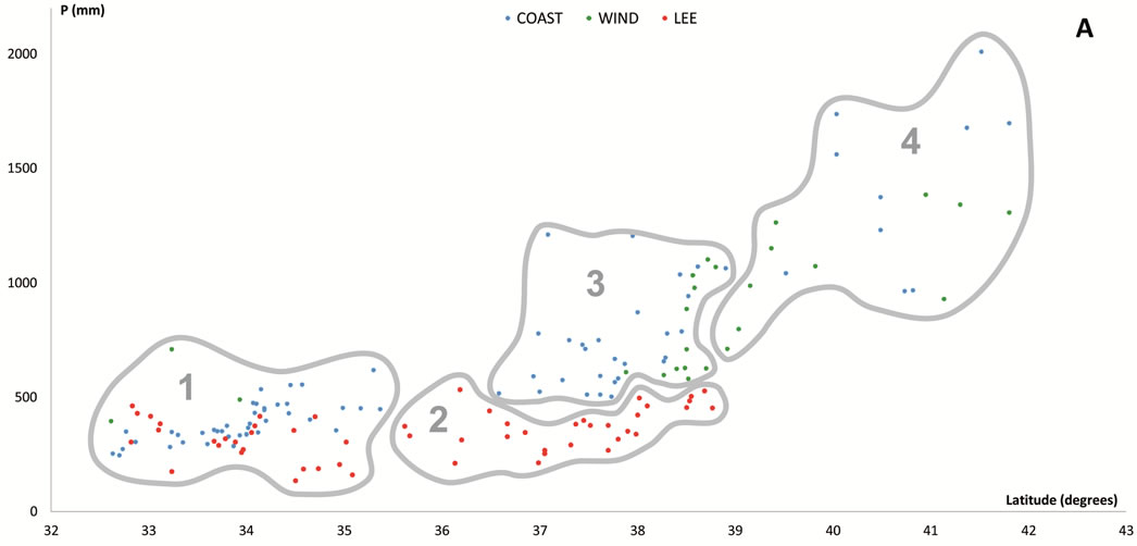
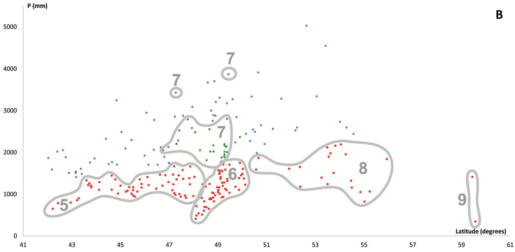
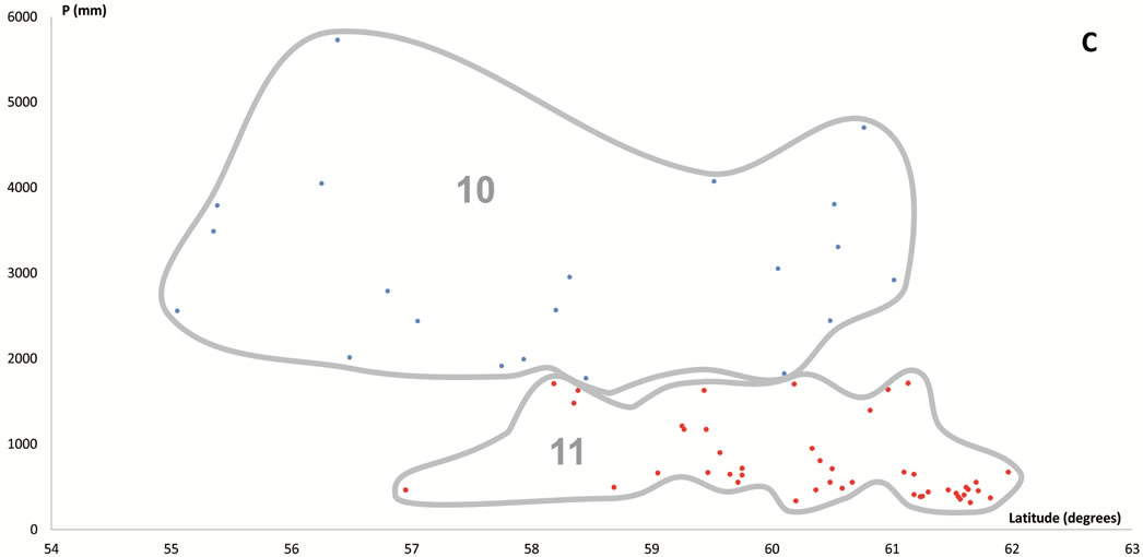
Figure 6. Scatter plots for 457 stations represented by their bioclimates. (A) Mediterranean stations: 1, Southern Coastal Ranges (1a: winward; 1b: leeward). 2, Central Coastal Ranges (2a: winward; 3b: leeward). 3, Northern Coastal Ranges. 4, Interior valleys of Oregon and Washington. 5, Puget Trough and Georgia Depression. (B) Temperate stations: 6, Northern Coastal Ranges and Cascades (6a: winward; 6b; leeward). 7, Vancouver Island (7a: winward; 7b: leeward). 8, British Columbia and Southern Alaska Coastal Ranges (8a: lowland stations; 8b: mountain stations). (C) Boreal stations: 9, Sitkan province (9a: windward of the Alaskan Coastal Ranges; 9b, leeward of the Alaskan Coastal Ranges and stations located inland, at the head of fjords). 10, Aleutian province. 11, Hudsonian province.
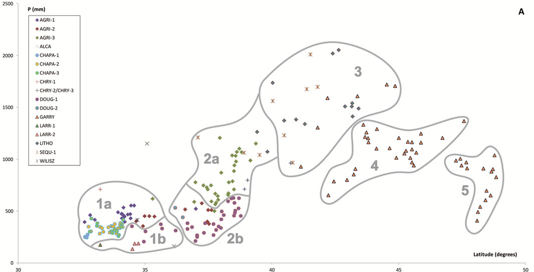
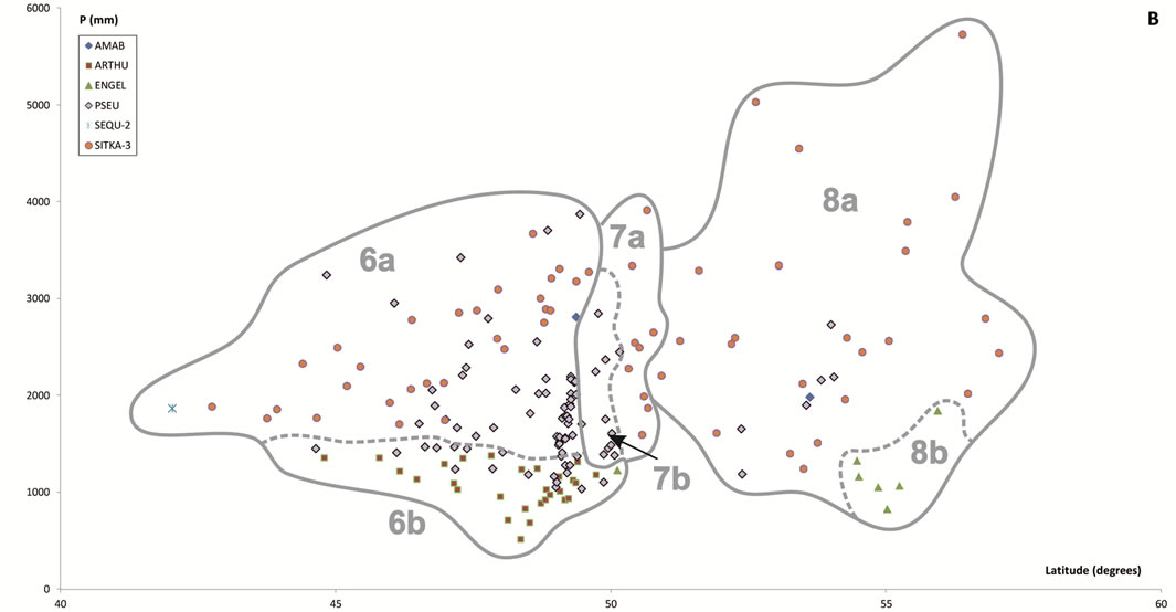
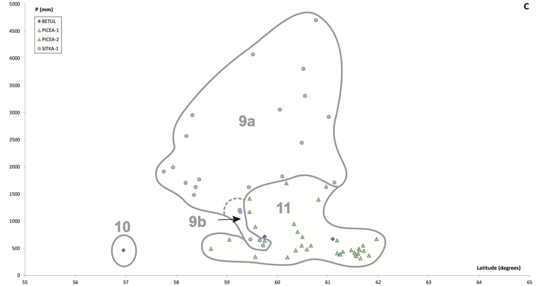
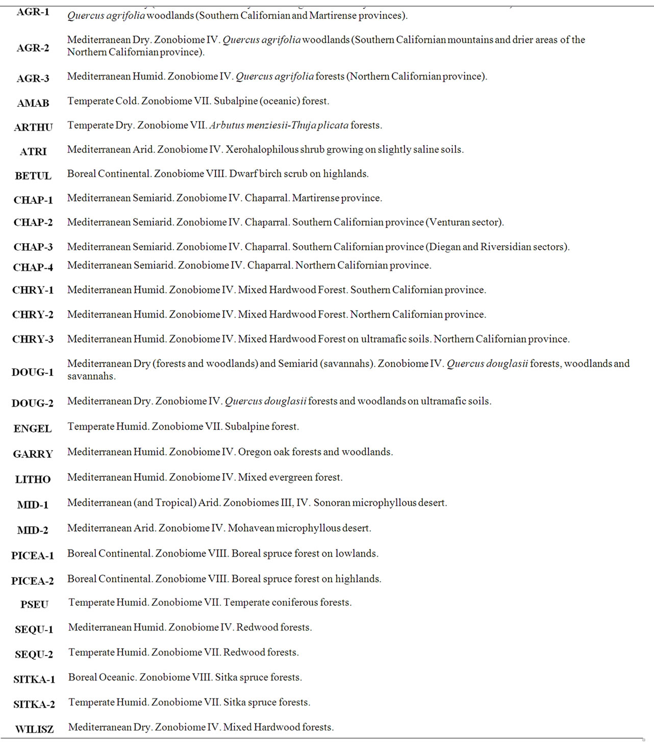
Table 4. Summarized descriptions (bioclimate, zonobiome or zonoecotone and brief diagnosis) of the vegetation types arranged alphabetically according to the abbreviations used in the text.
of the BC Coastal Ranges north of 58˚. Its presence is reflected by the appearance of Picea glauca forests and Picea mariana muskegs.
2) Sitkan, showing a Boreal Oceanic climate according to Walter’s classification or Mesothermal after Köppen’s system. The area spreads from coastal AK to approximately mainland Dixon Entrance, just north of the Queen Charlotte Islands, where the border with the temperate
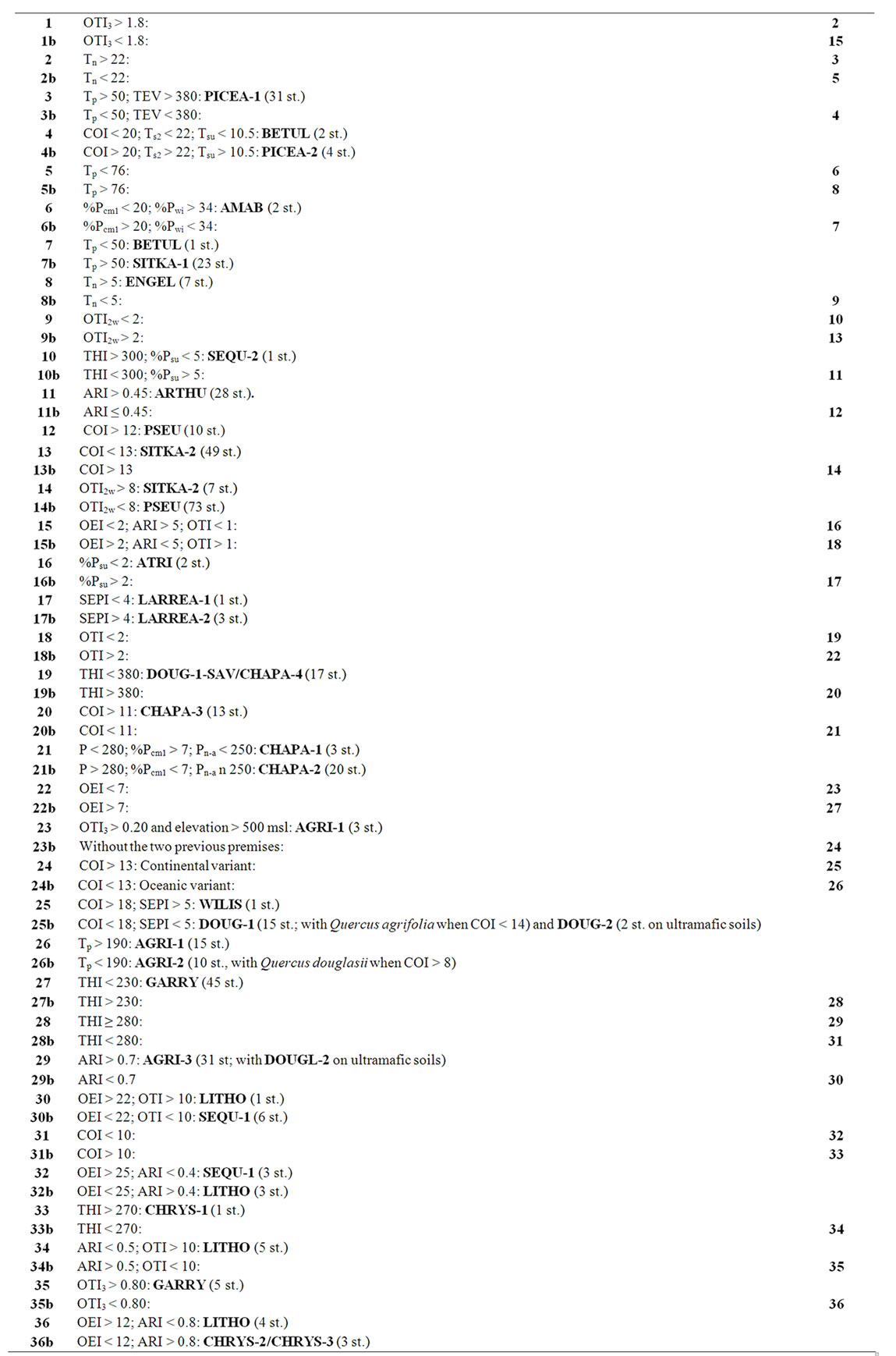
Table 5. Key to PNV types based on climatic differences. For abbreviations of climate data see Table 1, and for PNV see Table 4.
Table 6. Key to PNV types based on floristic and ecological differences. For abbreviations see Table 4.

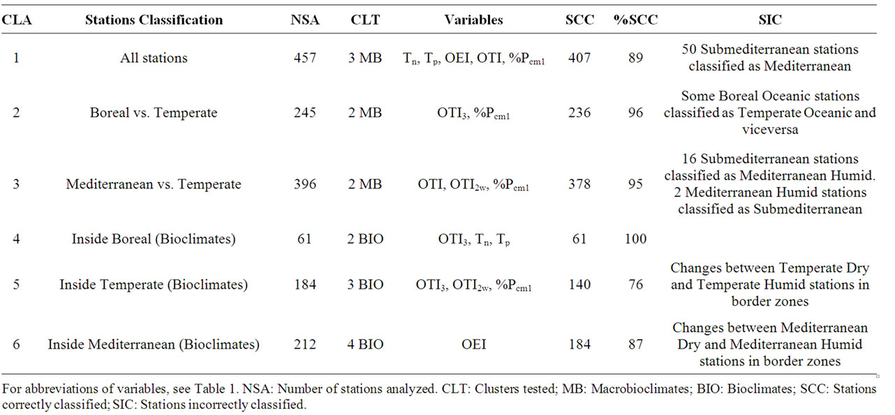
Table 8. Summary of the results obtained in the cluster analysis (CLA, k-means) for the six variables showing most significance (p < 0.0001). For abbreviations of climate variables see Table 1.
Oregonian province is found [11]. Sitka spruce forests constitute the PNV of this rainy and cold boreal coast.
3) Oregonian, spreading from Dixon Entrance southward, is a wide region in which the Temperate climate dominates until we reach the border between OR and CA. PNV in this province is dominated by typical temperate trees such as Abies amabilis, Picea sitchensis, Thuja plicata or Tsuga heterophylla.
The true boreal zone is recognizable in the climate diagrams as the point where the duration of the period with a daily average temperature of more than 10˚C drops below 120 days and the cold season lasts longer than six months [7]. Numerically, the best indices for discriminating boreal and temperate stations are negative (Tn) and positive (Tp) temperatures along with rainfall percentages during the warmest seasons (%Pcm1 and %Psu).
In the 79 northernmost and coldest stations Tn > 1. At 39 of these stations, located in inland Alaska zones colonized by taiga forests dominated or co-dominated by Picea glauca and/or P. mariana, Tn > 22. These were included within the Boreal Continental bioclimate. The remaining 40 northern stations can be divided into two groups. The first group includes 24 stations in cold regions (Tp < 76) with the highest or among the highest summer rainfall spread across the northern Alaska Pandhale. These stations were assigned to the Boreal Oceanic bioclimate. Also included in this group were two subalpine stations located above 850 msl in the British Columbia Coastal Ranges, but because both show lower summer rainfall values and their PNV is dominated by Abies amabilis, they can be easily included within the Temperate MB and their PNV is floristically related to other temperate forests. The second group comprises the remaining southern stations distributed in the southernmost part of the Alaska Pandhale and along the British Columbia Coastal Ranges, whose PNV is dominated by typical temperate species such as Picea engelmannii, T. plicata, T. heterophylla and P. menziesii, which never occur in the first group. This second group of stations was included in the Temperate Humid bioclimate.
Within the Mediterranean MB there are four bioclimates. Six stations sharing the highest values of aridity (ARI > 5 and OEI < 2) were included within the Mediterranean Arid bioclimate. Four of these located in southeastern California appear in the Mohave Desert, the most northwestern extension of the Sonoran Desert, a Tropical Arid zone lying in an area where Larrea tridentata dominates or co-dominates in every zonal community. The remaining two Mediterranean Arid stations are located further north, in the rainshadow of the Southern Coastal Ranges, in the driest parts of the Central Valley. At both stations, summer rainfall is three times lower and temperatures cooler, and their PNV (ATRI) is dominated by shrubs of the genus Atriplex, a feature of the climatophilous vegetation of the cold deserts of the Great Basin region [5].
There are two types of PNV in Mediterranean Semiarid areas: chaparrals and savannahs of Quercus douglasii. Chaparral, the evergreen sclerophyllous shrubland that dominates the cismontane side of coastal mountains ranges from about San Francisco south to Ensenada in Baja California, is the climatic climax in zones with Mediterranean Semiarid bioclimate and constitute degradation stages of sclerophyllous or mixed evergreen forests in areas of higher rainfall of both the Southern Californian and Martirense provinces [28]. In interior areas of the Northern Californian province, chaparrals (CHAPA-4) mostly pervade rocky places with shallow soils, while Q. douglasii savannahs (DOUG-1-SAV) seem to require deep phreatic layers, which can be reached by the powerful root system of the dominant tree [29,30].
In semiarid areas, Quercus agrifolia woodlands thrive only in gullies and canyons with access to additional soil moisture. The threshold 2 for OTI seems to be the best limit for discriminating Semiarid from Dry and Humid bioclimates. In dry or humid areas (OTI > 2), chaparrals may represent what remains after human activity has destroyed the trees. Otherwise, they are local seral brushlands on drier slopes with shallow soils; i.e., in such areas, chaparral is seral to the forest vegetation, not the natural climax. When OTI < 2, as in the Southern Californian and Martirense provinces, chaparrals are the true PNV.
Under the Mediterranean Dry bioclimate the PNV consists of oak forests and woodlands distributed according to continentality. In areas under maritime influence (COI < 13), the PNV comprises Quercus agrifolia forests and woodlands: AGRI-1, on warm lowlands (Tp > 190) of the Southern Californian province, and AGRI-2, inhabiting colder areas (Tp < 190) of the Southern Californian mountains and lowlands from Point Conception northwards. In continental areas (COI > 13), the PNV chiefly corresponds to Q. douglasii forests and woodlands: DOUG-1 thriving in normal, not ultramafic, soils, and DOUG-2, in ultramafic soils. In only one station showing the highest continentality index (COI > 18), the PNV is dominated by Q. wiliszenii (WILIS).
When precipitation increases and TEV decreases (OEI > 7), the Mediterranean Humid bioclimate occurs. Inland, mainly in the coldest (THI < 230) northern areas of Oregon, Washington and British Columbia, the PNV comprises Q. garryana forests and woodlands in wetter areas, or Q. garryana savannahs in the continental and drier valleys of central Oregon and Washington. These forests, woodlands and savannahs were here included within the vegetation type GARRY. Towards the coast, where temperatures rise (THI > 230), the PNV is mixed evergreen forests (LITHO), the classic broad sclerophyll forest described by Whittaker [31].
In the warmest areas across the windward slopes of the Coastal Ranges in central and northern California, the PNV is dense Q. agrifolia forests (AGRI-3). Unlike the southern oakwoods, those of AGRI-3 sustain a large group of differential taxa most of which also occur in northern forests such as LITHO and SEQU-1. From 35˚48' (at Salmon Creek, California), redwoods (SEQU-1) begin to appear. At the southern limits of their distribution area, redwood groves commence as isolated patches linked to riverbanks and shady canyons, such that between this latitude and 41˚ there exists a topographical mosaic, with redwoods settling on northern or ocean exposed slopes where the fog effect is ecologically important, and oakwoods, in contrast, thriving on sunny or leeward slopes.
The range of Q. agrifolia ends north of San Francisco Bay, and oak forests are replaced there by other mixed evergreen forests, mainly by LITHO, a Lithocarpus densiflorus-Arbutus menziesii forest, which appears on the Klamath and Siskiyou mountains on the northern California and southern Oregon coasts. This area is roughly coincidental with that of the redwoods (SEQU-1). There, LITHO is essentially a redwood border forest occurring mainly on sunny or leeward slopes, which receive less summer fog than the slopes sustaining redwood forests. In fact, both Whittaker [31] in the Siskiyou and Klamath, and Griffin [29] in northern California, refer to a Lithocarpus densiflorus-Arbutus menziesii forest that substitutes redwood forests according to a decreasing-humidity gradient. Inland, coastal trees such as L. densiflorus and Q. agrifolia do not flourish, and Quercus chrysolepis forests constitute the PNV in normal (CHRYS-2) and ultramafic soils (CHRYS-3). Only a mountain station in the Southern Coastal Ranges supports mixed forests dominated by the endemic Pseudotsuga macrocarpa (CHRYS-1).
Most of the floristic assemblages associated with redwoods can be divided into two groups; the northern group, closely related to the Oregonian floristic element, and the southern group, linked to the Californian floristic element [13]. These groups support two floristic and climatic redwoods: SEQU-1, of the Mediterranean Humid bioclimate, supported by many Californian elements, and SEQU-2, of the Temperate MB, differentiated by some Oregonian elements. This floristically intermediate composition between Mediterranean and temperate redwoods is consistent with Walter’s map [7, p. 12] in which the coastal border between California and Oregon is drawn as the ZE IV-V.
The most conspicuous feature of the temperate PNV of the Pacific Northwest with regard to other temperate forests of the world is the confining of deciduous trees to younger forests, riverbanks and frequently disturbed areas, and the dominance of giant conifers that escaped decimation during Pleistocene glaciation [32]. Although the PNV of the temperate areas is unified by climate and physiography and has an evergreen coniferous component, it varies from the coast inland, from south to north, from west to east and from low to high altitude.
From northern California, but principally from southern Oregon to the Gulf of Alaska, forests of Sitka spruce form a long narrow band adjacent to the Pacific ocean, where maritime influences are maximal, the temperature is cool and there is high precipitation and frequent fogs. Floristic and bioclimatic data suggest separating the Sitka spruce forests into two associations: SITKA-1, boreal, and SITKA-2, temperate, the latter grouping pervading forests from northern California to approximately Glacier Bay National Park in southeastern Alaska, where the SITKA-1 area begins and spreads northward to the sealevel timberline of P. sitchensis on the westernmost Kenai Peninsula of Alaska. Since the SITKA-2 distribution range occupies the area showing the greatest precipitation in western North America, the designations “perhumid rain forest” or “temperate rain forest” are generally used for these forests, while the boreal SITKA-1 has been called a “subpolar rain forest” [33]. Since the northernmost areas occupied by the SITKA-2 association are largely inaccessible, the northern limit of its range cannot be determined exactly; the transitional ecotone with the boreal SITKA-1 should lie somewhere between Glacier Bay and the Malaspina Glacier. As noted above, Walter [7] described this area as ZE V-VIII.
Away from direct oceanic influence, most of the temperate zone of the lowlands toward the interior of the coastal strip occupied by SITKA-2 is covered by mixed evergreen forests (PSEU), which correspond to the “temperate rainforests” so-called by American ecologists. From Oregon northward to southern British Columbia a less moist variant of PSEU predominates, the so-called “seasonal rainforest” [33], which is replaced inland eastwards, when OTI2w > 2, by the Submediterranean forests harboring Arbutus menziesii and Thuja plicata (ARTHU). The most humid variant, or “perhumid rainforest”, in which Abies amabilis is common and sometimes codominant with T. heterophylla and T. plicata, dominates low and medium elevations from northern Vancouver Island to Glacier Bay in northern southeast Alaska. At high elevations, subalpine forests (AMAB, in the Cascades; ENGEL, in the lee of the British Columbia Coastal Ranges) replace PSEU.
Within the Boreal MB there are two bioclimates. Along the rainier and foggier coasts of Alaska, windward of the Alaska-Chugach Ranges from Kenai south to approximately Yakutat Bay, appears the Boreal Oceanic bioclimate. The PNV corresponds to Sitka spruce forests (SITKA-1). Tsuga mertensiana and P. sitchensis dominate down to sea level, although the timberline can be as low as 200 m above sea level. T. plicata and P. menziesii, along with many other typical species of temperate forests were lacking in relevés taken in the SITKA-1 boreal forests.
The Boreal Continental bioclimate arises in the lee of the British Columbia coastal mountains north of 58˚. Its presence is reflected by the appearance of Picea glauca forests and P. mariana muskegs. This bioclimate spans most interior areas of British Columbia and Alaska, and only reaches the Pacific coast at Cook Inlet, in the lee of the Kenai coastal mountains, where the PNV mainly corresponds to a mixed deciduous-coniferous forest (PICEA- 1), which thrives in an area that is permafrost-free [10]. In contrast, PICEA-2 forests occupy zones where the ground is seasonally frozen, mainly in cryosols developed on north-facing slopes and higher altitudes. In permafrost-free, very dry soils (lithic regosols), mainly on rocky outcrops of the highest elevations, PICEA-2 alternates with BETUL, a woodland almost exclusively comprised of multistemmed and rather stunted Betula neoalaskana, which grow scattered among prostrate shrubs and over a dense carpet of fruticose lichens and xeric mosses.
5. Acknowledgements
This research was supported by grants from the Franklin Institute of North American Studies (University of Alcalá). The authors thank Ana Burton, who polished our English.
REFERENCES
- L. Brouillet and R. D. Whetstone, “Climate and Physiography,” In: Flora of North America Editorial Committee, Eds., Flora of North America: North of Mexico, Oxford University Press, New York, 1993, pp. 15-46.
- M. G. Barbour and W. D. Billings, “North American Terrestrial Vegetation,” 2nd Edition, Cambridge University Press, Cambridge, 2000.
- M. Peinado, J. L. Aguirre, J. Delgadillo and M. A. Macías, “Zonobiomes, Zonoecotones and Azonal Vegetation along the Pacific Coast of North America,” Plant Ecology, Vol. 191, No. 2, 2007, pp. 221-252. doi:10.1007/s11258-006-9239-8
- M. Peinado, M. A. Macías, F. M. Ocaña-Peinado, J. L. Aguirre and J. Delgadillo, “Bioclimates and Vegetation along the Pacific Basin of Northwestern Mexico,” Plant Ecology, Vol. 212, No. 2, pp. 263-281. doi:10.1007/s11258-010-9820-z
- S. Rivas-Martínez, “Syntaxonomical Synopsis of the North America Natural Potential Vegetation Communities, I,” Itinera Geobotanica, Vol. 10, 1997, pp. 5-148.
- S. Rivas-Martínez, D. Sánchez-Mata and M. Costa, “North American Boreal and Western Temperate Forest Vegetation,” Itinera Geobotanica, Vol. 12, 1999, pp. 5-316.
- H. Walter, “Vegetation of the Earth and Ecological Systems of the Geobiosphere,” 3rd Edition, Springer-Verlag, Berlin, 1985.
- S. Rivas-Martínez, S. Rivas-Sáenz and A. P. Merino, “Worldwide Bioclimatic Classification System,” Global Geobotany, Vol. 1, 2011, pp. 1-638.
- C. Ricotta, M. L. Carranza, G. Avena and C. Blasi, “Are Potential Vegetation Maps a Meaningful Alternative to Neutral Landscape Models?” Applied Vegetation Science, Vol. 5, No. 2, 2002, pp. 271-275. doi:10.1111/j.1654-109X.2002.tb00557.x
- M. Peinado, J. L. Aguirre and M. de la Cruz, “A Phytosociological Survey of the Boreal Forest (VaccinioPiceetea) in North America,” Plant Ecology, Vol. 129, No. 1, 1998, pp. 29-47. doi:10.1023/A:1009711818203
- L. R. Dice, “The Biotic Provinces of North America,” University of Michigan Press, Ann Arbor, 1943.
- M. Peinado, J. L. Aguirre, J. Delgadillo and M. A. Macías, “A Phytosociological and Phytogeographical Survey of the Coastal Vegetation of Western North America. Part I: Plant Communities of Baja California, Mexico,” Plant Ecology, Vol. 196, No. 1, 2008, pp. 27-60. doi:10.1007/s11258-007-9334-5
- M. Peinado, M. A. Macías, J. L. Aguirre and J. Delgadillo, “Fitogeografía de la Costa del Pacífico de Norteamérica,” Anales Jardín Botánico de Madrid, Vol. 66, No. 2, 2009, pp. 151-194.
- T. R. Karl and C. R. Williams, “An Approach to Adjusting Climatological Time Series for Discontinuous Inhomogeneities,” Journal of Climate and Applied Meteorology, Vol. 26, No. 12, 1987, pp. 1744-1763. doi:10.1175/1520-0450(1987)026<1744:AATACT>2.0.CO;2
- NOAA, “US Monthly Climate Normals 1971-2000,” US Department of Commerce, National Oceanic and Atmospheric Administration, National Climatic Center, Asheville, 2002.
- Ncdia, “National Climate Data and Information Archive,” 2003. http://climate.weatheroffice.gc.ca/climate_normals/index_e.html
- L. R. Holdridge, “Ecología Basada en Zonas de Vida,” Instituto Interamericano de Cooperación Para la Agricultura, San José de Costa Rica, 1982.
- S. L. Dingman, “Physical Hydrology,” 2nd Edition, Prentice Hall, Upper Saddle River, 2002.
- H. Ellenberg and D. Mueller-Dombois, “Aims and Methods of Vegetation Ecology,” John Wiley and Sons, New York, 1974.
- USDA, “The PLANTS Database,” June 2012. http://plants.usda.gov
- A. W. F. Edwards and R. A. Fisher, “Statistical Methods for Research Workers,” In: I. Grattan-Guinness, Ed., Landmark Writings in Western Mathematics: Case Studies, Elsevier, Amsterdam, 2005, pp. 1640-1940. doi:10.1016/B978-044450871-3/50148-0
- Z. Michalewicz and D. B. Fogel, “How to Solve It: Modern Heuristics,” Springer Verlag, Berlin, 2000.
- J. Hair, R. Anderson, R. Tatham and W. Black, “Multivariate Data Analysis with Readings,” Prentice Hall, Englewood Cliffs, 1999.
- W. R. Erickson and D. V. Meidinger, “Garry Oak (Quercus garryana) Plant Communities in British Columbia: A Guide to Identification,” Technical Report 040, British Columbia Ministry of Forests, Victoria, 2007.
- J. F. Franklin and C. Dyrness, “Natural Vegetation of Oregon and Washington,” 2nd Edition, Oregon State University Press, Corvallis, 1988.
- D. R. Thysell and A. B. Carey, “Quercus garryana Communities in the Puget Sound, Washington,” Northwest Science, Vol. 75, 2001, pp. 219-235.
- M. Peinado, F. Alcaraz, J. L. Aguirre and J. Álvarez, “Vegetation Formations and Associations of the Zonobiomes along the North American Pacific Coast,” Vegetatio, Vol. 114, 1995, pp. 123-135.
- M. Peinado, F. Alcaraz, J. L. Aguirre and J. Delgadillo, “Major Plant Communities of Warm North American Deserts,” Journal of Vegetation Science, Vol. 6, No. 1, 1994, pp. 79-94. doi:10.2307/3236259
- D. I. Griffin, “Oak Forest,” In: M. G. Barbour and J. Major, Eds., Terrestrial Vegetation of California, 2nd Edition, California Native Plant Society, Davis, 1988, pp. 383-416.
- J. Delgadillo, “Introducción al Conocimiento Bioclimá- tico, Fitogeográfico y Fitosociológico del Suroeste de Norteamérica Estados Unidos y México,” Ph.D. Thesis, Universidad de Alcalá, Alcalá de Henares, 1995.
- R. H. Whittaker, “Vegetation of the Siskiyou Mountains, Oregon and California,” Ecological Monographs, Vol. 30, 1960, pp. 279-338.
- R. H. Waring and J. F. Franklin, “Evergreen Coniferous Forests of the Pacific Northwest,” Science, Vol. 204, No. 4400, 1979, pp. 1380-1386. doi:10.1126/science.204.4400.1380
- J. Pojar and A. MacKinnon, “Plants of Coastal British Columbia,” Lone Pine Publishers, Vancouver, 1994.
Supplementary Material
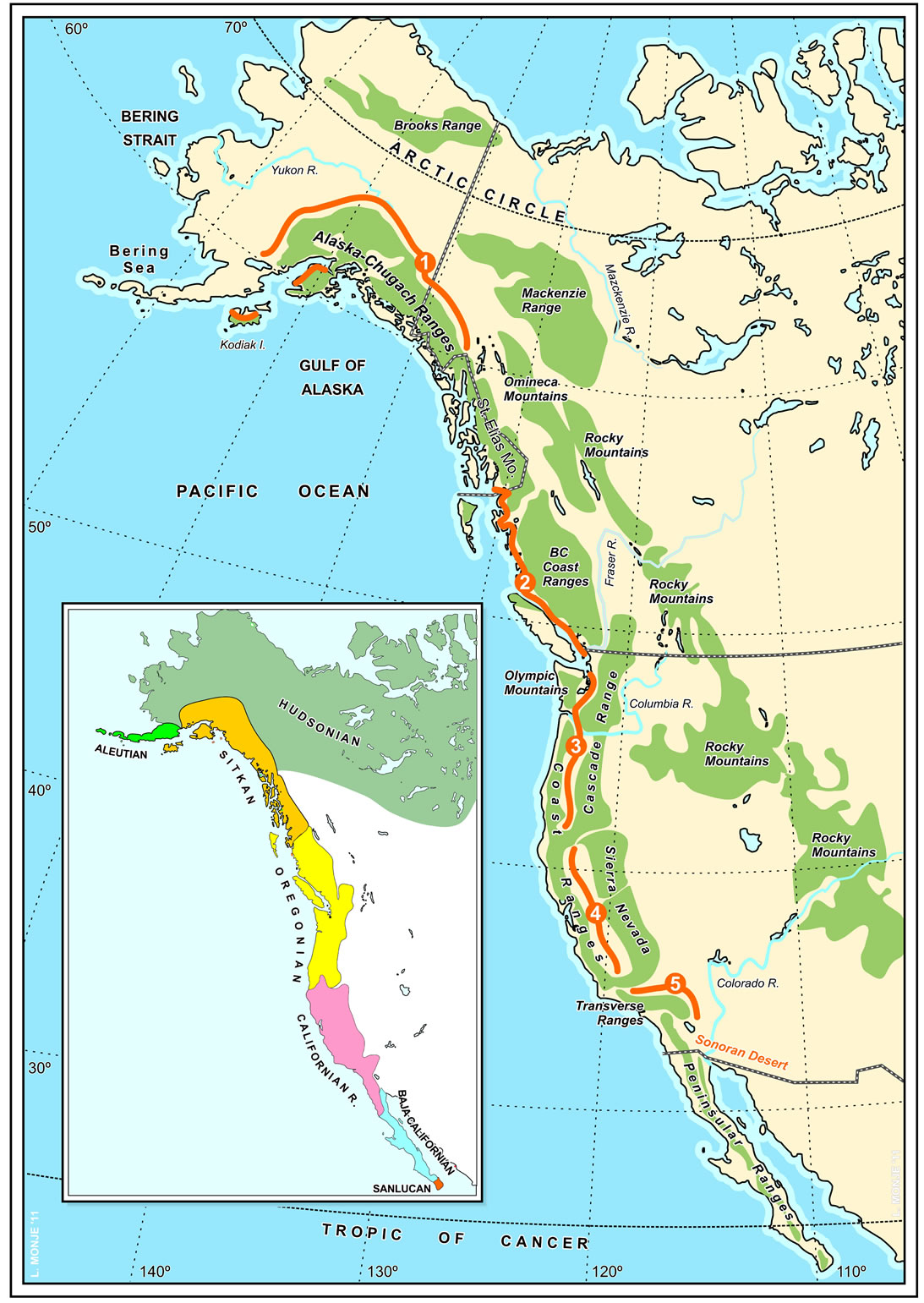
Figure S1. Physiographic map of the North American Pacific basin and phytogeographical units of the Pacific Northwest (lower left; after [11], slightly modified). Red lines mark the approximate location of the rainshadow areas: 1, AlaskanYukon plateaus and lee of the Alaskan ranges. 2, Alexander Archipelago-Nahwitti-Hecate-Georgia depressions. 3, Puget Trough and Willamette Valley. 4, Great Valley of California. 5, Mohave Desert.
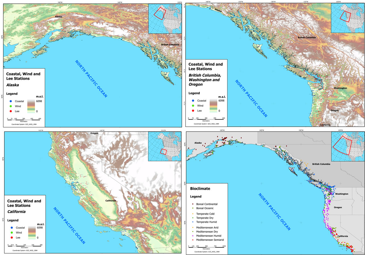
Maps S1 to S3 Coastal, wind and lee weather stations in Alaska (S1), British Columbia, Washington, Oregon (S2), and California (S3); Map S4 Bioclimates for 457 sampled stations.
Table S1. Climatic parameters and indices, bioclimatic classification, and PNV types for 457 sampled stations. For abbreviations of climate data see Table 1, and for PNV see Table 4. http://foto.difo.uah.es/geobotanica/ficheros/peinado/
NOTES
*Corresponding author.