Open Journal of Fluid Dynamics
Vol.2 No.4A(2012), Article ID:26352,7 pages DOI:10.4236/ojfd.2012.24A030
Characteristics of Unsteady Boundary Layer Induced by the Compression Wave Propagating in a Tunnel
Department of Energy and Environmental Engineering, Graduate School of Engineering Sciences, Kyushu University, Fukuoka, Japan
Email: 2ES11175N@s.kyushu-u.ac.jp
Received September 15, 2012; revised October 27, 2012; accepted November 6, 2012
Keywords: Transition; Unsteady Boundary Layer; Compression Wave; Laser Differential Interferometry
ABSTRACT
A compression wave is generated ahead of a high-speed train, while entering a tunnel. This compression wave propagates to the tunnel exit and spouts out as a micro pressure wave, causing an exploding sound. In order to estimate the magnitude correctly, the mechanism of the attenuation and distortion of a compression wave propagating along a tunnel must be understood and experimental information on these phenomena is required. An experimental and numerical investigation is carried out to clarify the mechanism of the propagating compression wave in a tube. The final objective of our study is to understand the mechanism of the attenuation and distortion of propagating compression waves in a tunnel. In the present paper, experimental investigations are carried out on the transition of the unsteady boundary layer induced by a propagating compression wave in a model tunnel by means of a developed laser differential interferometry technique.
1. Introduction
Many transfer phenomena of the wave motion of the compressive fluid in the pipe can be confirmed in the industry. For instance, operating the air brake equipment in the car, and opening rapidly the valve or rupturing the pipe in gas pipe line, it becomes unsteady flow with a compression wave and expansion wave in the pipe tube.
In these days, it becomes the problem of a pressure wave propagating in the pipe. It occurs that a lot of noisy problems affect the health in our life. For example, the exhaust sound generates the open end of exhaust pipe when rotating in high speed the engine of the automobile with high output power. It sounds like scrunching such as shaking the metal plate, this sound is very harsh. It is required to clarify the mechanism of propagating the pressure wave generating from the vent of engine to the exhaust pipe exit.
By the way, for a pressure wave, there are a shock wave, a compressional wave, and various things including an expansion wave. In this study, we focus on the compression wave as seen in many cases on the Industrial problem. Therefore, we give an example of compression wave propagating through the tube as an Industrial problem.
This example is the process that a high-speed train passes through the tunnel. When a high-speed train entering a tunnel, train compresses the air in front of a train like a piston effect, compression wave is formed as shown in Figure 1. This compression wave propagates to the tunnel exit and spouts out as an impulsive wave, causing an exploding sound. This impulsive wave is called a “micro pressure wave” [1]. This micro-wave makes doors and windows of nearby buildings shake, and this sound may make many problems of our health in daily life because of including a very low frequency ingredient, lower than 20 [Hz]. And, it is confirmed that the magnitude of this exploding sound can be almost proportional to the square of the speed rush of the train to the tunnel, so this sound prevents improving train’s speed-up. And, according to the aeroacoustic theory, the magnitude of a micro pressure wave is proportional to the maximum rate of the pressure change of the pressure change of the pressure wavefront at the tunnel exit [2]. Also, it is more required that the mechanism of attenuation and distortion of a compression wave propagating along a tunnel must be understood in order to reduce this tunnel noise and estimate this magnitude correctly. In addition, it is needed to experimental information on these phenomena.
A lot of experimental and numerical research of the compression wave propagating in the pipe has been carried out [3,4]. However, these studies are often considered the propagation characteristics focused on the wavefront the compression wave front. In order to clarify the
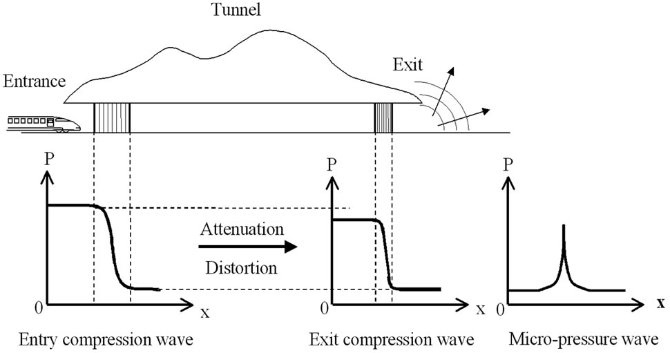
Figure 1. Developmental mechanism of micro-pressure wave.
propagation characteristics of compression wave properly, it is necessary to consider the attenuation and distortion of the backward wave front, for instance unsteady boundary layer developed behind the compression wave.
In this paper, we generate a compression wave in a tube of constant cross section with a wave motion simulator and measure unsteady boundary layer developing behind a compression wave by Laser Differential Interferometry; LDI. It is the primary purpose to capture a flow induced behind compression wave and to consider the characteristics of unsteady boundary layer.
2. Experimental Procedure
2.1. Experimental Apparatus
The detail of wave simulator used in the experiments is shown in Figure 2. This experimental apparatus is composed of a fast opening gate valve instead of a filmbreaking device of normal shock tube, described in 1993 by Aoki et al. It is composed of wave driving unit (highpressure chamber), fast opening valve, tube wave propagation (low-pressure chamber, test section). The highpressure chamber is circle pipe, made of PVC, 4 [m] length, 76 [mm] diameter, filled the air as a driving gas. The low-pressure chamber is rectangular pipe, made of stainless steel, 7 [m] length, 56 [mm] × 56 [mm] crosssection, open-ended to the air. Test section is fitted up at 3900 [mm] from the fast opening valve, and pressure sensors for pressure measurement are installed at 750 [mm] and 3900 [mm] from the valve. Optical glass is installed on the side of test section, and a laser beam is penetrated in low pressure chamber pipe through this glass.
Next, a schematic diagram of the optical arrangement of laser differential interferometry for measuring the flow behind the compression wave is shown in Figure 3. A continuous He-Ne laser is used as a light source and is converted the linearly-polarized laser into circularlypolarized light by retardation plate. The circularly-po-
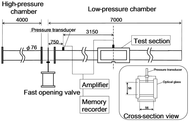
Figure 2. Detail of a wave simulator.
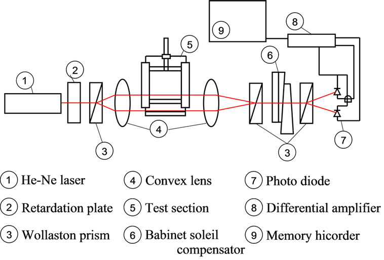
Figure 3. Optical arrangement of laser differential interferometry.
larized laser is divided for two linearly-polarized laser beams that polarization plane is perpendicular each other next by first Wollaston prism. These laser beams are divided between the reference beam and test beam by convex lens. The test beam penetrates measurement object, and is occurred optical path difference by density variations for reference beam. Two beams are recombined by the second lens and the second Wollaston prism. These beams seem to be one beam, but do not yet interfere because they are polarized perpendicular to each other. And, it can be regulated the phase of these two beams polarized perpendicularly each other by the Babinet-soleil compensator. These beams are separated by third Wollaston prism and irradiate photo diodes. Photo diodes used for two detecting the difference of light intensities. The difference of the two detector signals from LDI will therefore be essentially free from vibrations and laser output variations. The difference of light intensities is finally converted to the voltage by the circuit of photo diode, and voltage difference is taken by the differential amplifier. LDI can be made more sensitive to optical path change by 2 to 3 orders of magnitude than classical interferometry. The sensitivity was high enough to record density variations of a compression wave. The origin of the x is distance of 750 [mm] from the fast opening valve. This LDI has been used to detect the transition region in the unsteady boundary layer at x = 3150 [mm], and test section is also installed at x = 3150 [mm]. A compression wave at x = 0 [mm] is the initial pressure waveform, and compression waveform distorted in propagating in a pipe is measured at x = 3150 [mm].
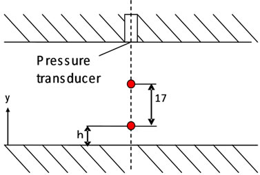
A schematic diagram of the optical setup of laser beam in test section is shown in Figure 4. This experiment is carried out as three LDI setups as shown in Figures 4 (a)-(c). In the case of setup A, one of the interfering laser beam (test beam) passes through the inside of tube. The other beam (reference beam) travels through the outside of pipe. In the case of setup B, one of the interfering laser beam (test beam) passes through the unsteady boundary layer at a height; h. The other beam (reference beam) travels through the main stream of the flow. In the case of setup C, two beams travel at the same height; h. Therefore setup A shows absolute density of the tube, and the output signal of setup B shows the difference of density between the boundary layer and main stream.
 (a)
(a)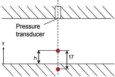 (b)
(b)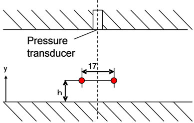 (c)
(c)
Figure 4. Schematic diagram of optical setup of laser beam. (a) Setup A; (b) Setup B; (c) Setup C.
Setup C is used to measure the spatial difference history of density. In each setup, it is measured in changing the height; h = 1, 2, 5 [mm].
2.2. Experimental Conditions
Initial conditions are shown in Table 1. In each condition, the compression waveforms propagating in test section at x = 3150 [mm] are shown in Figure 5. In the case of condition C and D, we can confirm overshoot of the pressure.
3. Result and Discussions
In this chapter, we discuss the characteristics of the unsteady boundary layer to measure the density of the tube by LDI, developed behind the compression wave.
3.1. Density Measurement in the Tube
In the case of setup A, Figure 6 shows as converted an output measured value of LDI into density. It is shown the results of measurement at height; h = 2 [mm], 5 [mm] in Condition C, and the theoretical value when assuming isentropic change.
The density increases with the passage of the compression wave, grows closer to the wall. This is because of the influence of the boundary layer closer to the wall. In addition, the density has fluctuated over time also after passing the wavefront. It is considered that the flow behind compression wave is non-stationary.
3.2. Relative Density with the Main Stream
In the case of setup B, Figure 7 shows as converted the
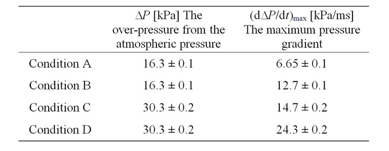
Table 1. Initial compression waveform.
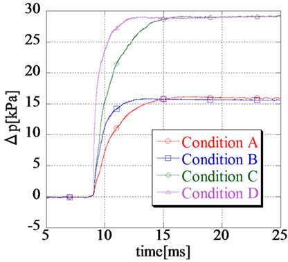
Figure 5. Propagating compression waves.
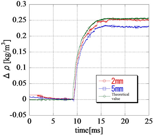
Figure 6. Measured density profiles in rectangular tube (Setup A).
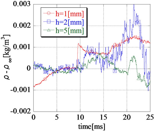
Figure 7. Measured density profiles in rectangular tube (Setup B).
measurement results into density. Figure 7 is result in condition C. We discuss about the wavefront after passing through due to the change in density before passing the wavefront by the fast opening valve of friction and vibration. In all cases the height from the wall; h = 1 [mm], 2 [mm] and 5 [mm], the density increases as time passed after passing the wavefront, but the increasing density decreases once. It is thought that a decrease region of the density appeared since the boundary layer profile has changed from laminar flow to turbulent flow, in other words boundary layer has transitioned. It is considered that the time to turn for decrease is s start of transition and the time to turn for increase again is an end of transition.
3.3. The Spatial Change in Boundary Layer
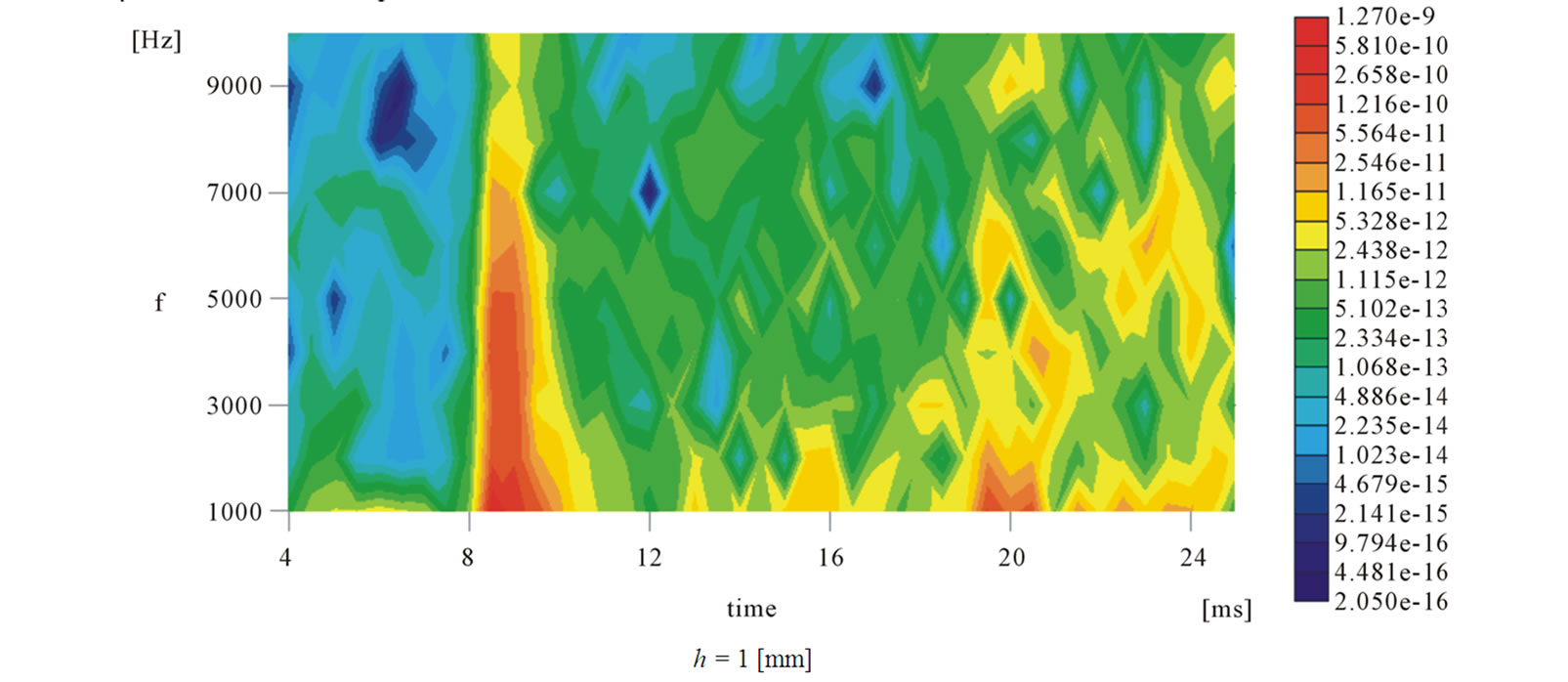
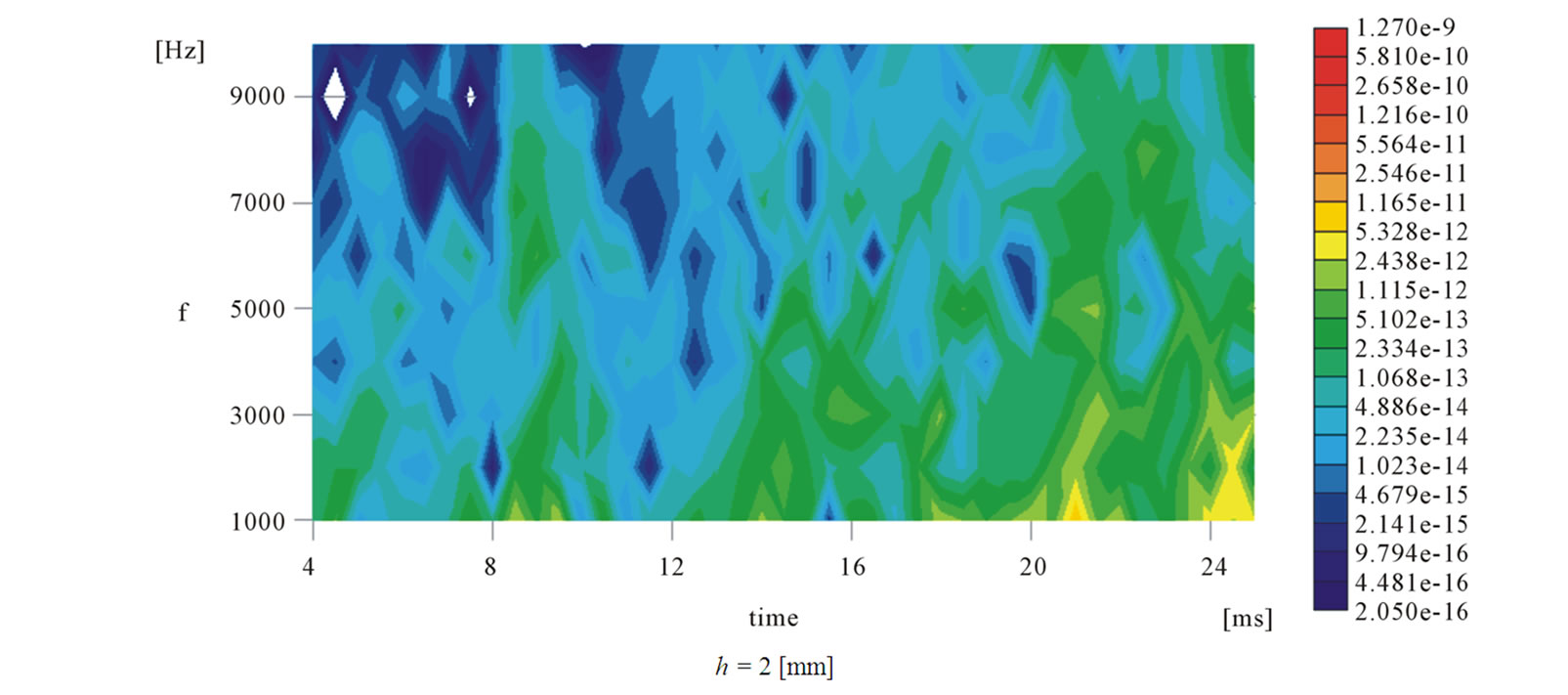
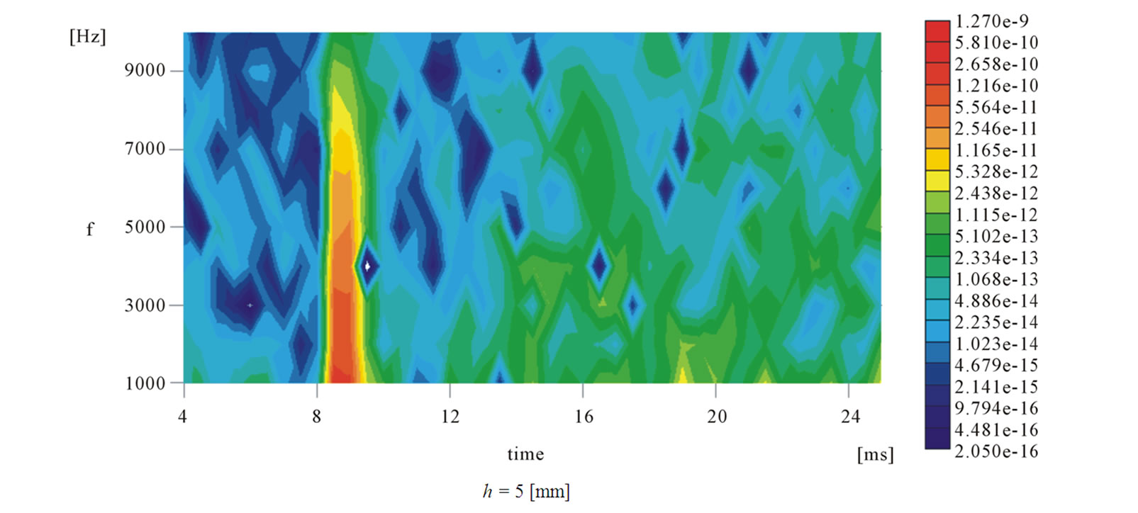
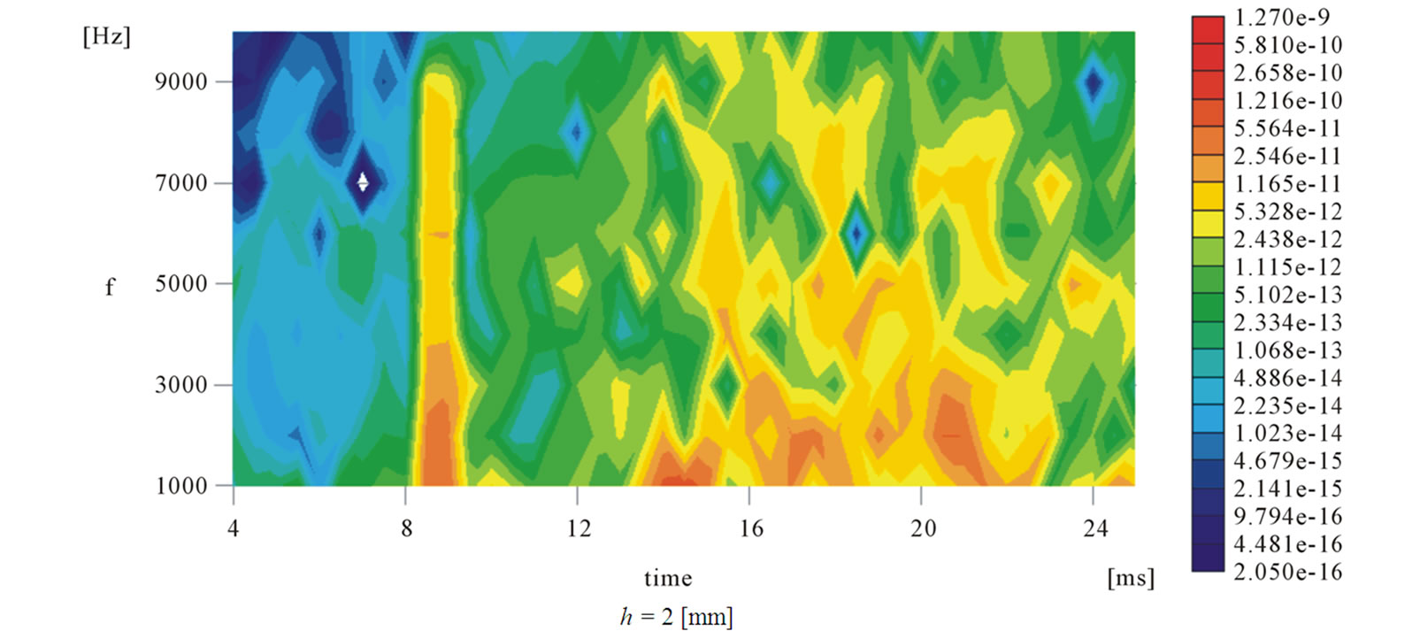
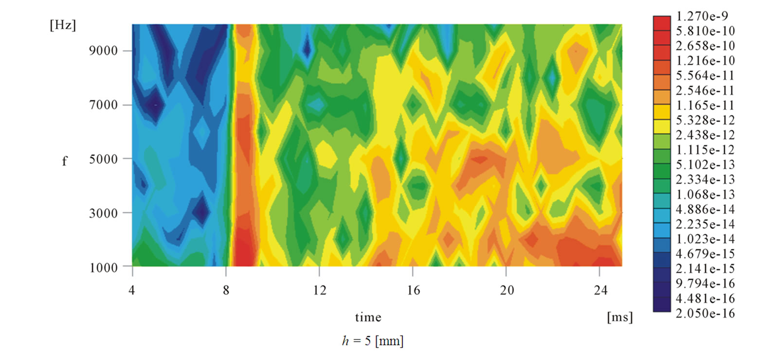
In the case of setup C, Figure 8 shows the experimental result in Condition D at the height from the wall; h = 1 [mm]. The voltage rapidly changes by passing the compression wave. Figure 9 shows distribution diagram of Power spectral density, PSD [(kg/m3)2/Hz] which converts the output by LDI into density and carried out short-time Fourier transform, STFT. Figure 9(a) shows distribution in condition B, Figure 9(b) shows in condition D, and the vertical axis is frequency [Hz], the cross
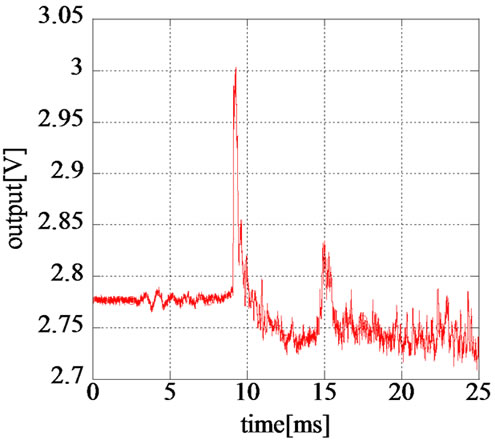
Figure 8. Output signal from LDI (Setup C).
axle is time [ms]. PSD suddenly increases after passing the wavefront at height; h = 1 [mm], but it does not rise very much at height; h = 2, 5 [mm] in Figure 9(a). In the case of Figure 9(b), PSD increases after passing the wavefront at all height; h = 1, 2, 5 [mm]. Also, PSD increases less than frequency (about 3 [kHz] in condition C) that divides flow speed induced behind the compression wave by beam spacing, i.e. 17 [mm]. This is caused by the fact that there is micro-flow speed disturbance which is less than speed of flow behind the compression wave.
3.4. The Transition of Unsteady Boundary Layer
Figure 10 shows the time variation of sum of power spectral, PSP [(kg/m3)2] which integral PSD in the range of 3 - 8 [kHz] in Figure 9. In condition D, we can confirm overshoot of pressure waveform and we calculate the time; ∆ttr1, ∆ttr2 shown below in Table 2. This time in the range of PSP in Figure 10 has a broad peak. In other words, the transition region is considered to be the area of this peak. We introduce transition Reynolds number; Retr [-] from a study of Hartunian with this time; ∆ttr1, ∆ttr2 [6].
 (1)
(1)
We substitute ∆ttr1, ∆ttr2 for ∆ttr and demand Retr1, Retr2. This result is shown in Figure 11. The vertical axis is Reynolds number [-], the cross axle is the maximum pressure gradient of initial compression wave [kPa/ms]. The initial compression wave intensity increases, the transition Reynolds number increases in Figure 11. In addition, the initial maximum pressure gradient increases the transition Reynolds number decreases. When we compare influence of both on transition Reynolds number, transition Reynolds number takes influence of the initial compression wave intensity than the pressure gradient of initial compression wave greatly.
4. Result and Discussions
In this study, we measure using LDI for the flow behind
 (a)
(a)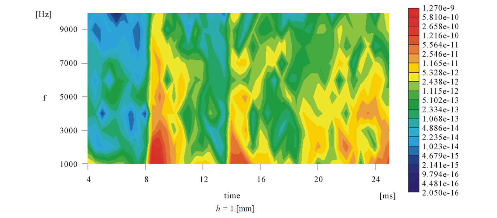
 (b)
(b)
Figure 9. Short-time Fourier transform of LDI. (a) Condition A; (b) Condition B.
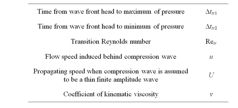
Table 2. Numerical conditions.
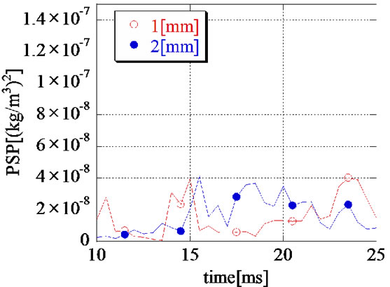
Figure 10. Sum of power spectrum between 3 [kHz] and 8 [kHz] (Condition D).
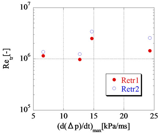
Figure 11. Transition Reynolds number of unsteady boundary layer.
compression wave to propagate in a rectangular tube.
1) By placing the laser in the horizontal direction, we can obtain change in the boundary layer profile;
2) When it changes the profile in the boundary layer, PSD rapidly increases in frequency domain calculated from beam spacing and flow speed behind the compression wave by the frequency analysis of density change;
3) Influence on transition Reynolds number of initial compression waveform is greater the initial intensity than the pressure gradient of initial compression wave.
REFERENCES
- S. Ozawa, T. Maeda, T. Matsumura and K. Uchida, “Countermeasures to Reduce Micro-Pressure Waves Radiating from Exits of Shin-Kansen Tunnels,” Proceedings of 7th International Symposium on Aero-Dynamics and Ventilation of Vehicle Tunnel, Elsevier Science Publishers Ltd., London, 1991, pp. 253-266.
- H. Kashimura, T. Yasunobu, T. Aoki and K. Matsuo, “Emission of a Propagating Compression Wave from an Open End of a Tube,” JSME International Journal Series B, Vol. 39, No. 3, 1995, pp. 475-481.
- K. Matsuo, T. Aoki, H. Kashimura, M. Kawaguchi and M. Takeuchi, “Attenuation of Compression Waves in a High-Speed Railway Tunnel Simulator,” Proceedings of 7th International on Aero-Dynamics and Ventilation of Vehicle Tunnel, Elsevier Science Publishers Ltd., London, 1991, pp. 239-253.
- T. Fukuda, S. Ozawa, M. Iida, T. Takasaki and Y. Wakabayashi, “Distortion of the Compression Wave Propagating Through a Very Long Tunnel with Slab Tracks,” JSME International Journal Series B, Vol. 71, No. 709, 2005, pp. 36-43.
- S. Nakao, “The Propagating Characteristic of Weak Pressure Wave in Long Tube,” Doctoral Dissertation, Kyushu University, Fukuoka, 2000.
- R. A. Hartunian, “Boundary-Layer Transition and Heat Transfer in Shock Tubes,” Journal of the Aerospace Science, Vol. 27, No. 8, 1960, p. 587.