American Journal of Industrial and Business Management
Vol.3 No.1(2013), Article ID:26800,10 pages DOI:10.4236/ajibm.2013.31012
Performance Evaluation for Pull-Type Supply Chains Using an Agent-Based Approach
![]()
1Department of Industrial, Manufacturing and Systems Engineering, The University of Texas, Austin, USA; 2Business Analytics, University of Phoenix, Phoenix, USA; 3Department of Information Management, National Chi Nan University, Nantou, Chinese Taipei.
Email: btseng@utep.edu, roger.gung@phoenix.edu, cchuang@ncnu.edu.tw
Received July 12th, 2012; revised September 28th, 2012; accepted October 30th, 2012
Keywords: Supply Chain Management; Pull Type; Supply Chain Model; Make-to-Plan; Agent Technology; Simulation
ABSTRACT
The business world changes rapidly and customers’ demands are more varied than before, traditional push system which takes actions based on anticipated requirements and uses forecast to determine the manufacturing quantity is no longer effective enough for modeling market volatility. Therefore, the pull strategy, which is demand oriented, flexible and generates cost savings, is becoming more popular and prominent. The pull type supply chain management is also applied broadly in the high-tech industry where the market volatility is a very unique characteristic. In SCM, nonstructured oral communications make information sharing difficult and inefficient in a distributed environment. To solve this problem, Agent Technology (AT) is applied. AT in Business Intelligence (BI) has been proven that it is good tool in solving communication problems in distributed environments. This research focuses on the application of the Make-to-Plan (MTP) supply chain strategy and AT based technique. A case study of simulation of the MTP-based pull type supply chain is presented. Impacts of operator parameters, e.g., manufacturing throughput, forecast accuracy, and inventory on performance of the pull type control strategies are discussed in this study.
1. Introduction
The essentials of Supply Chain Management (SCM) is a set of practices aimed at managing and coordinating the Supply Chain (SC) from raw material suppliers to the ultimate customer [1]. SCM includes activities such as planning, product design and development, sourcing, manufacturing, fabrication, assembly, transportation, ware-housing, distribution, and post delivery customer support [2]. There are two typical types of the SC models from the viewpoint of material control: push and pull types. The pull strategy, which is demand oriented, flexible and generate cost savings is becoming more popular and prominent [3]. Furthermore, the pull type supply chain management is applied broadly in the high-tech industry where the market volatility is a very unique characteristic. Companies such as Dell, HP, IBM, and Philips are attempting to adapt this type of the SC model to respond to the agile business world [4].
In the viewpoint of demand management, one of the most employed requirements planning in the house-ware industry is make-to-plan (MTP) since consumer electronic products contain less degree of modularity over the PC industry and the WIP is of less value, where the make-to-order (MTO) strategy is mainly applied [5]. Therefore, the house-ware industry may try to achieve the lower inventory and prefers on demand forecasting to preserve low inventory and reduce unexpected waste. The house-ware industry prefers to ignore the strict zero inventory requirement in order to save on transportation costs. Furthermore, consumer electronic products are relatively less expensive than computer products and the market is less volatile as well. A higher degree of uncertainty of sales and longer lead time for delivery of raw materials are also anticipated. Most of the pull type systems related literatures focus on make-to-order (MTO) strategy and the models pursuit of zero inventory [6], cycle time reduction [7], lead time reduction [8], and on time delivery [9]. However, few literatures are focused on MTP study, specifically the impacts of operation parameters in SCM, e.g., throughput, forecast accuracy, demand variability management, and safety level stock to on the performance of a SC to take advantages of the pull type control strategy.
Moreover, a supply network is a system that is characterized by complexity, randomness, dynamics and limited transparency. The complexity has its roots in the high number of partners, the number of links and relations among them, as well as the response time (delay). The supply chain as a whole system seems to be not transparent from the point of view of an individual enterprise, because of the inability of this company to collect all relevant information in the required quantity and quality (accuracy) [10]. The fluctuation in demand amplification causes a growth of the costs and a decrease of the service through higher stock levels, a greater fluctuation of quantities and a rise of the complexity of scheduling [10]. Also, non-structured oral communications in a SC do not make information sharing easy and efficient any more.
To solve these problems, agent technology (AT), which is capable of performing a specific task without direct human supervision and communicating with other agents is applied. It is because that AT is a good tool in solving communication problems in distributed environment.
This research focuses on the application of the MTPbased strategy and the agent technology. Impacts of manufacturing throughput, demand variability management, and safety stock on the pull type performance, the performance of AT on forecast accuracy improvement and simulation of the MTP-based pull type supply chain are discussed in this study. The remaining paper is organized as follows: Section 2 provides the related literature reviews. Based on comparison of the push and pull strategies in SCM, a modified MTP-based pull type SC model is proposed in Section 3. The novel SC control policies, supply planning and inventory planning, are also created in response to market competition. Section 4 illustrates a simulation model to verify the proposed approach and explore the aforementioned impact. Section 5 concludes this paper.
2. Literature Review
The supply chain models are divided into a push type and a pull type according to the flow of information. From the perspective of demand management, the pull type approach is classified into MTO order-oriented strategy and MTP, a market demand (plan) oriented strategy.
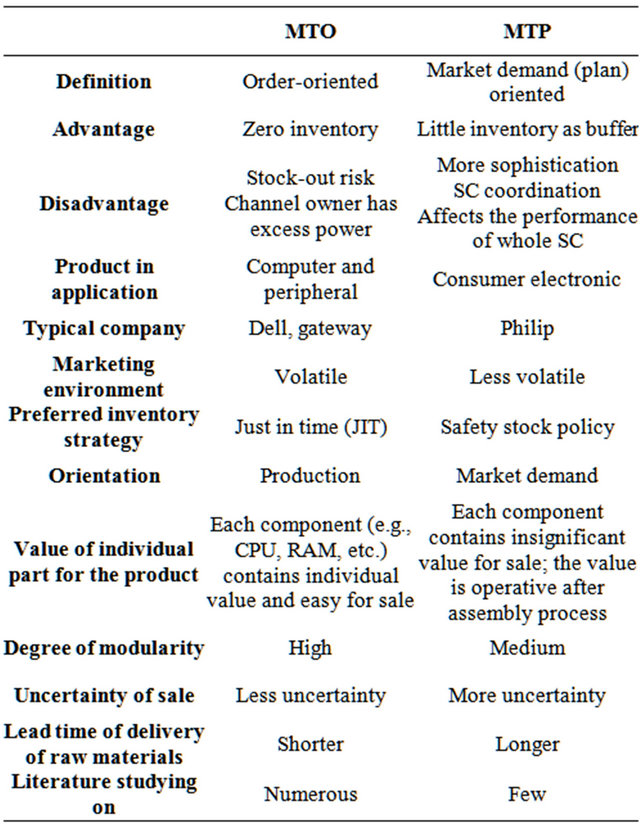
Literatures focusing on MTO based pull type model explores (develops) zero inventory [11], lead time policy [12], pricing [13], and agility [14] and postponement [15]. MTP refers to manufacturing according to plans. A plan refers to sophisticated calculation of forecast according both to past historical consumption and possible future change inputs from the market. In addition, MTP decides on the desired level of factory utilization and acquires components to produce and maintain that level. Literatures focusing on the MTP-based pull type model explores manufacturing process [16], computerization [17], process planning [18], information sharing [19], integrated [20]. Consequently, few literatures are focused on MTP study. Table 1 summarizes the characteristics of MTO and MTP.
An important part of agent technology is the principle which agents can function more effectively in groups that are characterized by cooperation and division of labor. Agent programs are designed to autonomously collaborate with each other in order to satisfy both their internal goals and the shared external demands generated by virtue of their participation in agent societies [21].
Although literatures and empirical applications do demonstrate the advantage of the MTO-based pull type SCM, few literatures explore the MTP-based pull type SCM. For example, there is no explicit testing of the influences such as SC design change on operation parameters like lead time, throughput, inventory level, and other factors mentioned above. Therefore, a MTP-based pull type SC is presented and discussed in this research. Basically, the impacts of throughput, safety stock, forecast accuracy, manufacturing validated line item effectiveness on total cost, penalty charge, fill rate, and on-time delivery rate in this system are studied in this paper. Since most events in a MTP-based pull type SC are discrete in nature, consequently simulation becomes a good tool to analyze effects of individual actual change and cross effects
Table 1. Comparison of MTO and MTP.
of the various factors. Without any reservation, simulation is the first-priority method in our case study. Through the simulation analysis, the results are capable to indicate the impact that every different variables cause toward to the entire supply chain to determine the best model for enterprises.
Furthermore, agent technology is an exciting new approach of creating complex software systems [21]. A variety of definitions of agents are offered by researchers and practitioners [22]. For example, Yang et al. (1999) define an agent as a program that is capable of performing a specific task without direct supervision from human [23]. Using agent technology can solve the issues relevant to difficulties and inefficiencies of information sharing in a distributed environment and provide insightful recommendations to allow the policymakers to make prompt decisions and therefore operation cost reduction can be achieved.
3. Proposed the Make-to-Plan (MTP)-Based Supply Chain Strategy
This research proposes a MTP based supply chain strategy, which incorporates the implementation of agent technology. Section 3.1 introduced a make-to-plan pull type supply chain model. Section 3.2 proposed the architecture of agents in the supply chain model. The formulism for the MTP based SC strategy is presented in Section 3.3.
3.1. Supply Chain Model
This study looks into a three-echelon supply chain with one product item which comprises final manufacturers, distribution centers, and retailers. The final manufacturers in different places in the world send the products to the distribution center close to the market place and the products are sent to the required retailer. In the pull supply chain, the production is based on the need of the succeeding echelon. That is, the retailer passes the orders to the distribution center, and the distribution center requests the manufacturer for products. In this approach, the inventories can be minimized and storage cost can be saved.
In the proposed make-to-plan, the manufacturer first makes certain manufacturing plans according to the historical data and the possible demand variation information from the retailer. The manufacturing preparation processes begin ahead of the actual demand, but communications with the retailer never stop. On the other hand, the retailers have their own selling strategies to plan their possible demand. They pass their possible demand to the manufacturer and distribution center so that the manufacturer can adjust the production plan if required. At a certain time point, the retailer has to confirm the demandwhich means that the order enters the frozen period. Once confirmation is received only then does the manufacturer enter the final stage of production. After the production phase, the finished goods are sent to the distribution center and then shipped to the retailer.
3.2. Agent in the MTP Supply Chain
As Hinkkanen et al. (1997) has suggested, agents can be modeled as humans who accommodate different situations [24]. Therefore, the supply chain can be completely driven and managed by agents. The goal of agents here is to share information with the three echelons to enhance communications and to provide better transparence in order to reduce uncertainties in forecasting.
The agent system architecture is shown in Figure 1. All of manufacturers (Mfgs.), distribution centers (DCs), and retailers (WRtlrs) provide their inbound and outbound quantities, time, and other necessary information to the rule base. For a Mfg., the production schedule, strategy and information, are also provided. For a Rtlr, the actual demand, planned activities, sales, and strategies are all sent to the rule base.
All of the inputs in the rule bases are then transformed into useful data when computing the forecast in the demand forecast agent. The forecast calculated in the demand forecast agent will be sent to the control agents in the three echelons to compute different data needed in the echelon. For a Mfg., the production plan will be calculated by its control agent and passed on to different stations in the manufacturer. For a DC, the forecast from demand forecast agent will be transformed into data needed for ordering. For a Rtlr, the demand forecast agent passes the same possible demand to the DC as it sends to the Mfg., any modification to the demand will
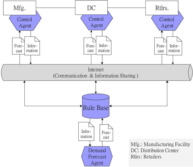
Figure 1. Agent system architecture.
The agents involved in the pull type SC play four roles:
A scheduler is an agent that schedules the synthesis of jobs which this agent responds to.
A manager is an agent that communicates with other agents and maintains the database where desired information for agent jobs is stored.
An optimizer is an agent that optimizes the synthesis based upon the requirements and constraints from downstream demand.
An explorer is an agent that searches the parts that are located in other distributed databases.
All agents have the same basic architecture: This involves an agent body that is responsible for managing the agent’s activities and interacting with peers and an agency that represents the solution resources for job synthesis problems. The body has a number of functional components responsible for each of its main activities—scheduling job synthesis, optimizing product synthesis, searching desired parts, and managing databases. This internal architecture is broadly based on the Grate [25] and Archon [26] agent models.
The domain resources include not only databases and job synthesis, but also other agents. The latter case allows a nested (hierarchical) agent system to be constructed in which higher-level agents realize their functionality through lower level agents (the lower level agents have the same structure as the higher level agents and, can, therefore, have sub-agents as well as synthesis jobs in their agency). For example, the higher level agent may represent a product design department whose work is carried out by a number of design teams (the lower level agents). This structure enables flat, hierarchical, and hybrid organizations to be modeled in a single framework. This modeling ability is important because commercial environments are founded on organizational models where an enterprise is logically divided into a collection of services. The agent-agency concept draws upon this principle to group services and jobs where it is pragmatic. The differences between an agent in an agency and a peer agent associated with the levels of autonomy are an agent in an agency implements the jobs depending on the request from the manager in the agency while a peer agent is autonomous without any imposing order from others. In both cases the agents negotiate to reach agreements— however in the former case: 1) the agent cannot reject the proposal outright (although it can counter-propose until an acceptable agreement is reached); and 2) the agent must negotiate in a cooperative (rather than a competitive) manner (since there is some degree of commonality of purpose). In summary, there is a tight coupling between an agent and its agency, and between an agent and its peers in two ways: loosely coupled and tightly coupled. In a loosely coupled interaction each agent has an equal status, no one agent controls another. In tightly coupled mode, one agent is a controlling agent and the other agents have access restricted from agents outside of the agency [27]. Next, the formulism to optimize SC operations through a control agent is presented.
3.3. Formulism for the MTP-Based SC Strategy
According to the production planning of MTP, two major issues are presented as follows: Supply planning, which focuses on changes or modifications in work-in-process or production parameters such as yields and cycle times. Sense-and-Respond monitors supply versus demand and capacity utilization to provide key reports when demand is in jeopardy and help understand the impact of the tardiness. This information enables analysts to gauge anticipated supply against demand by demand class, immediate identification of demands in jeopardy, identify assets supporting this demand, and full profile of anticipated capacity utilization [28]. On the other hand, inventory planning, which plays a role as a buffer to absorb the uncertainties through the supply chain environment, focuses on changes in a business policy such as inventory days of supply which is also impacted by changes in manufacturing practice such a shorter cycle times. The inventory management process controls the manufacturing of wafers, devices, and modules based on inventory reorder points [28].
3.3.1. Supply Planning
In the proposed MTP supply chain, the supply plans are made by the DC every week. In order to pursue low inventory throughout the whole supply chain, finished goods are sent to the DC for distribution as soon as possible and get to the retailers right on time to fulfill the need. A DC plays a critical role in MTP supply chain. Whether the fill rate and on-time delivery are achieved or not depends a lot on the manufacturing release time it demands from the manufacturing site. Therefore, the supply plan is modeled for a product model manufactured in a manufacturing site and shipped to a DC.
In pull strategies, “on-time” plays an important role. Products are expected to be manufactured on time for delivery to the DC. And the DC is expected to give the wholesales the needed amount of products on time for selling. Two important time points are thus considered into the supply plan: lead time and frozen period. Frozen period(s) is the time period within which changes to the supply plan are not permitted. For example, for the next x weeks, the supply plan is frozen as input to the manufacturing planning and execution; Mfg.-DC lead time (L) is average lead time from the start of manufacturing to receipt at the DC (i.e. number of weeks needed for the product to flow through manufacturing). The last few weeks of lead time is frozen period.
In the supply plan on-hand inventory, safety stock, demand forecast, and the average expected receipt together determine the amount of manufacturing release requirement. The accumulated demand forecasts for week i, I + 1, …, I + L minus the accumulated expected receipt for week i, I + 1, …, I + Z − 1, minus on hand inventory and plus the safety stock for I + Z week equals to the manufacturing release for week i. The detailed calculations are illustrated as follows:
 (1)
(1)
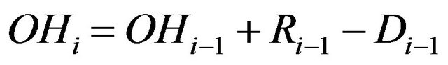 (2)
(2)
 (3)
(3)
where Z: frozen periodL: lead timeMRi: manufacturing release requirement for week iFi: demand forecast for week iERi: expected receipt for week iERi: the average ERiOHi: beginning on-hand inventory level at week iSSi: safety stock level for week iRi: total actual receipt during week iDi: total actual demand during week i.
As shown in Equation (1), the demand forecast must be done for week i, i + 1, …, i + z before releasing the manufacturing requirement for week i. Forecasting indeed plays an important role in supply planning, and in this research we define the factors influencing demand forecast for week i include: the actual demand for the last week (Di−1, D~N ), market uncertainty (
 ,
, ~N(
~N( ,
, )) which is the most unpredictable and technology improvement uncertainty (
 ,
, ~N (
~N ( ,
, )) that will likely make accurate forecast inaccurate.
It is clear in Equation (2) that on-hand inventory is calculated as the on-hand inventory last week plus actual receipt last week and minuses the actual consumption for last week.
Furthermore, in Equation (3), although ideally the real receipt of week i + L equals to the manufacturing release requirement for week i that is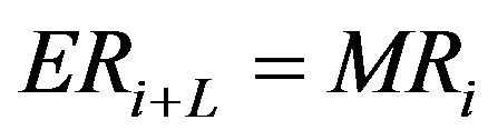 , but due to the various causes of uncertainties, the ideal situation may not hold. Thus, we use the average of the expected receipt over a long period of time
 , which is normally distributed to construct the new MR. As to the difference between
  and
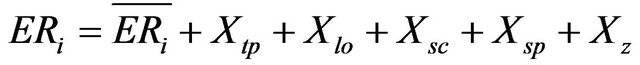
and , it will be absorbed by safety stock which is normally distributed as well. The causes of the difference might be due to several uncertainties illustrated as follows:
Transportation (Xtp): the driver may get lost due to wrong direction; the incidents like traffic jam or car accident may occur during the trip.
Unidentified loss (Xlo): this might be caused by loss of product due to theft or human counting error, etc.
Supplier in-time capability (Xsc): once the demand excesses the normal demand too much, the supplier may not have enough capability to produce the required amount, or even the supplier’s financial situation might affect the production.
Uncertainty of the supplier’s suppliers (Xsp, Xsp ~(μsp, σ2sp)): the relationship of the supplier and its suppliers may be out of the control span and thus causes uncertainties.
Uncertainty caused by frozen time (Xz, Xz ~exp(μz)): the chance of changing the order gradually freezes within the frozen time. The frozen period has an exponential distribution. However, since the demand may not be fully forecasted, the frozen time enlarges the risk caused by the above uncertainties.
All the above uncertainties except for Xz are normally distributed, thus:
 (4)
(4)
The distribution of  is the combination of normal distribution and exponential distribution.
3.3.2. Inventory Planning
Inventory plays a role as a buffer to absorb the uncertainties through the supply chain environment. However, various inventory costs (i.e. opportunity cost of capital, loan interest, taxes and insurance cost, cost for handling and storing the inventory, and possible cost of lost, stolen, damaged, or obsolete inventory) make firms seek to minimize inventories. To reduce the aforementioned costs and uncertainties, the safety stock policy is applied. Safety stock is the basic amount of inventory that must be kept in the warehouse. The more precise the safety stock level is, the better cost control the firm is capable of. As the safety stock level takes into consideration during manufacturing release, the supply planning can be more beneficial and accurate from the safety stock level.
To determine the safety stock, the service level must be confirmed. Then the safety stock is calculated as demand over L + 1 weeks ( ) plus target service level
  times standard deviation of demand over L + 1 weeks
  adding the aforementioned uncertainties. For easier understanding, X is proposed here to represent the sum of all uncertainties.
 (5)
(5)
Note that the first six uncertainties are normally distributed, the sum of them is a multi-normal distribution,
With XZ, the distribution of X is the combination of multi-normal and exponential distribution. So that the safety stock (SS) policy is illustrated as:
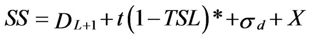 (6)
(6)
Also,
 (7)
(7)
In conclusion, for OHi, Ri−1 and Di−1 are normally distributed, it also has the form of normal distribution. Furthermore, the distribution of MRi is

which is also the sum of normal and exponential distribution. Equation (3) shows that ERi has the same distribution as MRi.
Next, the performances of the proposed plan making methodology are implemented in the simulation process as follows in Section 4.
4. Simulation of the MTP-Based Pull Type Supply Chain
The proposed methodologies are demonstrated and validated by empirical data using simulation. The simulation model is developed in Section 4.1. The simulation results are presented in Section 4.2. Section 4.3 concludes this simulation study.
4.1. Simulation Model
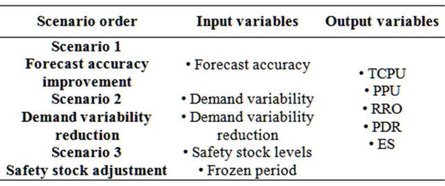
In this model, four performance factors are investigated in this simulation to explore the components of the MTPbased pull type supply chain in practical: 1) forecast accuracy improvement; 2) demand variability management; and 3) safety stock. Note that the safety stock is perceived as a buffer. The simulation focuses and intends to validate on the following studies:
Forecast accuracy improvement is the expected effect through applying agent technology (Scenario 1).
Demand variability management enhancement represents better coordination throughout the supply chain and the effects of demand variability reduction is investigated (Scenario 2).
Safety Stock is needed in MTP as mentioned in Section 3.3. Therefore, the attempt to define the optimal safety stock level is investigated in the research (Scenario 3).
In the first scenario, forecast accuracy is investigated. Forecast accuracy is a rate which represents accuracy of the customer’s forecasts. It is calculated as the average of the absolute deviation of the forecast from the actual orders, expressed as a percentage error. As concerning forecast accuracy, it is anticipated that the application of agent technology (AT) can enhance forecast accuracy rate, and the improvement caused by the AT is expected to affect all dependant variables. In the first simulation scenario, agents are added in the model. In this model, each manufacturer, DC, and retailer include control agents performing different tasks. In addition, in the simulation, the impacts of forecast accuracy improvement by applying AT on total cost per unit (TCPU), ratio of received and ordered (PRO), prompt delivery rate (PDR), estimated savings ($K) (ES), fill rate (FR), and on-time delivery rate (OTR) are surveyed.
Three manufacturers (Mfg.-1, Mfg.-2, and Mfg.-3) with different frozen periods are selected for the experiment due to the following reasons: first, different distances to the North American market, which is the major market in the model; second, diverse transportation/shipment uncertainty exists; third, there is different manufacturing flexible levels are anticipated. The product type selected for this investigation is a video since for its product characteristics is less complexity.
While in the second scenario, demand variability management is investigated. Demand variation is the variation of the demand within a month, calculated as standard deviation divided by mean demand then the calculated value times 100. Since AT is capable of improving communication through the whole supply chain thus improve coordination to reduce demand variation, the effects of demand variation reduction is of interest. It is expected that better demand variation management can result in better fill rate and on-time delivery rate and less penalty cost.
At last, safety stock level is investigated in the third scenario. Two products, video and Light Emitting Diodes (LED) television, are used as an example and discussed in the example. In general, video product is less complex than LED in production process. Different items are added to the week of supply (WOS) to examine the impacts on the dependant variables. The objective of this operation is to determine the best inventory level for the products.
In the Arena model, an agent is assigned in each Mfg., DC, and Retailer and plays four roles presented in Section 3.2. Basically, the simulation is replicated 1024 times. The statistics functions are always reset and the system is set to empty every replication (iteration). The simulation reports reflect the 273 days of each replication. The time unit for reporting in the simulation is “hour”.
All data for the listed input variables are from the historical data given by the case company. Through the interactions of input variables by scenario settings, the changes of the output variables are investigated. The goal of pursuit the minimum cost leads to the investigation on total cost. However, though cost reduction is the goal of most manufacturing facilities, business satisfaction in modern business is receiving growing attention. Not only fill rate but on-time delivery rate is investigated in the research. The penalty cost provides an overall view in the ability of making customer contented with the production and delivery. Therefore, in all scenarios the output variables include Total cost per unit (TCPU); Penalty per unit (PPU); Ratio of received and ordered (RRO); Prompt delivery rate (PDR); Estimated savings (ES) ($K).
Despite the common input/output inbound variables, such as inbound/outbound transportation cost, warehousing cost, lead time, and so on, the specific variables applied in each scenario are listed in Table 2.
4.2. Simulation Results
All simulation scenarios are compared with the current status, which is defined as a “Baseline” (Case B-0), without launching the agent technology. The simulation results are shown next.
• Scenario 1—Impacts of forecast accuracy enhancement At the first stage of this scenario, case F-1, agent technology is applied to the supply chain model. The prediction accuracy is indeed enhanced to approximately 60%. With the prediction accuracy level, total cost per unit is reduced by $0.08, penalty cost per unit is $0.04 reduced. “Ratio of received and ordered” and “prompt delivery rate” are enhanced by 2% and 1% respectively. The estimated savings is $112,000 per week. Even agent technology is proven to be working; the effectiveness is not significant in this study in case F1.
The idea of the second stage experiment is to identify the impact of further improvements in prediction accuracy. At this stage, the prediction accuracy is assumed to be 70%, 80% and 90% in the simulation settings (Cases F2, F3, and F4). This is to test whether further improvements on prediction accuracy is worthy. The assumption lies in the possible efforts in agent technology such as implementing neural or artificial intelligence. Though the implementation is not discussed in this research, the performance on further improvements is simulated as a
Table 2. The relationship between key input/output variables and the scenarios.
comparison to the proposed agent technology. The interest of this stage lies in the impacts on the dependant variables. However, as the prediction accuracy is improved, stock-out risks may increase since in practical SS may be reduced. Since this risk is not specified in the experiment, it is necessary to raise safety stock level in order to compensate for increased stock-out risk. As higher prediction accuracy rate may accompany higher stock-out risk, 0.1 week of supply (WOS) safety stock level goes with 70% and 80% of prediction accuracy rate while 0.8 WOS is assigned to 90% of prediction accuracy rate.
When prediction accuracy rate achieves 70%, it is coupled with $0.23 and $0.08 reductions in total cost per unit and penalty cost per unit respectively. In this case F-2, the ratio of received and ordered is 2% higher, and the prompt delivery rate is same as the current situation. When prediction accuracy rate achieves 80%, coupled with 10% WOS added to safety stock level, total cost per unit is $0.40 reduced and prompt delivery rate is 1% lowered. However, the penalty cost per unit is higher than the current system, and ratio of received and ordered is 1% enhanced. This may result in from the insufficient safety stock. The result in case F-3 leads to a higher safety stock level in case F-4. The forth case F-4, which is the most costly among the three cases, combines the methods proposed in the first and second cases. In the third case (F-3); a group of experts are added and the frequency of prediction is twice per week. Moreover, the safety stock level is 0.8 weeks of supply higher than the present level. The prediction accuracy is expected to achieve 90% and both total cost per unit and penalty cost per unit are expected to have $0.83 and $0.25 reduction. The increase of “Ratio of received and ordered” and “prompt delivery rate” are both 2%. The projected savings, $922,000, is much higher than the former two cases. However, with 80% of prediction accuracy and additional 0.1 WOS, the penalty cost per unit is $0.1 higher than the baseline value. This effect may be accrued from risk of stock-outs.
In the first simulation scenario, it is known that agent technology indeed helps improving customer forecast and that also improves forecast. In conjunction with adding safety stocks, it can help reduce costs and improve service.
• Scenario 2—Impacts on demand variability management
In pull strategy, information sharing throughout the supply chain can bring synergies to the whole supply chain. Each firm on the supply chain collaborates with each other, and shares better demand variability management. In this scenario, the effect of demand variability management is tested. The simulation shows that reduced demand variability can save total cost and penalty cost (TCPU). “Ratio of received and ordered” (PRO) is 2% improved when demand variability is 40% reduced. If demand variability is 10% reduced then prompt delivery rate (PDR) is improved by 1%. In conclusion, developing a collaborative approach for demand planning/ management can lead to unit cost reduction of 0.5% and improve ratio of received and ordered.
• Scenario 3—Impacts of safety stock
In supply chain design, the determination of safety stock level is an art. Redundant inventory increases manufacturing cost; there is stock-out risk if too little inventory. This scenario provides an investigation in the video and LED safety stock levels for the retailer.
The result for LED is obvious and clear. Increasing the safety stock level with 1 WOS can reduce both total cost and penalty cost, but with increased “ratio of received and ordered” and “prompt delivery rate”. When increasing safety stock level with 2 WOS, unit cost is $0.28 increased (from $85.02 to $85.3) without improvement in “ratio of received and ordered” and “prompt delivery rate”. Therefore it can be seen that the best safety stock level for the retailer is one WOS more than the current safety stock level.
For video, the situation is more complex than expected. From the perspective of total cost and projected savings, the best safety stock level is 3 WOS increased; from that of the penalty cost, “ratio of received and ordered” and “prompt delivery rate”, the best level is 4 or 5 WOS increased. In this case study, service performance can be improved by increasing safety stock levels in video and the safety stock levels must be carefully defined in order to avoid excess costs.
The simulation results show that increasing safety stock levels improves fulfillment performance for penalty charge going down and both “ratio of received and ordered” and “prompt delivery rate” increase because of safety stock increment. For total cost per unit, it decreases up to a certain level. However, safety stock increases alone cannot help achieve 100% ratio of received and ordered and inventories cannot be reserved for specific customers. Inventory analysis tool should be exercised to determine overall safety stock levels.
4.3. Simulation Result Remarks
In Section 4.2, the simulations of agent technology, forecast accuracy improvement, demand variability reduction, and safety stock level adjustments have be conducted by comparing the effects on unit total cost, unit penalty cost, projected savings, fill rate, and on-time delivery rate. The results of the scenarios have shown that the application of Agent Technology can help forecast accuracy improvement. And that the further pursuit of forecast accuracy improvement is capable of lowering penalty cost yet requires additional safety stock. The effects of demand variability reduction are shown. At the last scenario, the effects of safety stock level adjustments are shown. Table 3 shows the comparison of estimated earnings for all scenarios and cases.
Here, several key input-output relationships were observed in this company. These relationships are unique and specific to this research. In general, simulation results in numerous solutions, due to the limitation of the size of this paper, only the most critical solutions were shown. For example, when throughput is increased, inventory cost goes up, but penalty charge goes down. Quantity produced is increased and so is quantity shipped. As shortened frozen period is coupled with increased throughput, inventory cost, penalty charge, and produced quantity decrease, but shipped quantity goes up. When base stock is increased, inventory cost surely goes up, and penalty charge is decreased. The produced and shipped quantity simultaneously goes up. When forecast accuracy is improved, base stock can be lessened and result in lower inventory cost, production quantity and shipping quantity. However penalty charge might increase. When lower base stock level and better forecast accuracy are achieved simultaneously, inventory cost and production quantity are not changed while penalty charge decreases and shipped quantity increases. When demand variability is lowered, probability due to alliance, inventory cost and penalty charge may lessen and production and shipped quantity may increase. When flexible fulfillment policy is applied, only inventory cost goes down, the other three factors, penalty charge, quantity produced and quantity shipped, all go up. The summary of the key relationships is illustrated in Table 4.
The simulation analysis suggests that key conclusions regarding the supply chain performance are as follows:
• Improving customer forecasting and demand behavior helps reduce costs and improve service. Demand variability (particularly within a month) can be influenced by customer collaboration and promotions.
• Built-to-Order Policy leverages improvements in different supply chain components to improve overall performance.
Table 3. ID’s respect to cases.
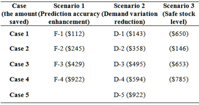
Table 4. Key input-output relationships.
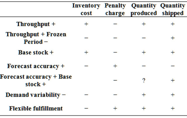
Note: “+” sign denotes increase; “−” sign denotes decrease; and “?” sign denotes uncertainty.
• Safety stock levels need to readjusted and maintained to ensure customer service. However, safety stock increases have marginal returns after a point and by themselves cannot achieve 100% service.
• As safety stock levels are increased, total costs go down and then go up. To optimize total costs, safety stock levels need to be set at this point. As the optimum setting shifts based on demand (size and variability) and other factors, this needs to be adjusted frequently.
• Adjusting the supply chain levers in combination provide maximum savings at realistic improvement targets.
In summary, Table 4 above provides useful information for the pull type MTP SC to capture multiple correlations between input and output variables.
5. Conclusions and Future Studies
This study has proposed a MTP-based pull supply chain strategy and provided a real data case study about the effects of throughput improvement, forecast accuracy improvement, demand variability management, and safety stock level adjustment on total cost, penalty cost, fill rate, and on-time delivery. Also, agent technology is applied in this research to investigate its effects on forecast accuracy performance.
A MTP-based pull strategy in SCM is novel in SCM since related research is not as sufficient as expected. Moreover, agent technology is an emerging technology which requires more insight and expertise in the field. Future research directions can focus on:
• Investigation on more dependant variables: In this research, total cost, penalty cost, fill rate and on-time delivery rate were investigated. However, other dependant variables such as quality, bathe size, transportation cost, etc. are also important in SCM. So further investigations are anticipated.
• Exploration of different forecast mechanisms using agent technology: Currently, many new mechanisms in the calculation of forecast such as genetic algorithm (GA), fuzzy set theory, are available. It is promising to combine the aforementioned approaches and agent technology to achieve better performance in forecast accuracy.
REFERENCES
- J. Heikkilä, “From Supply to Demand Chain Management: Efficiency and Customer Satisfaction,” Journal of Operations Management, Vol. 20, No. 6, 2002, pp. 183-193. doi:10.1016/S0272-6963(02)00038-4
- K. C. Tan, “A Framework of Supply Chain Management Literature,” European Journal of Purchasing & Supply Management, Vol. 7, No. 1, 2001, pp. 39-48. doi:10.1016/S0969-7012(00)00020-4
- M. C. Bonney, Z. M. Zhang, M. A. Head, C. C. Tien and R. J. Barson, “Are Push and Pull Systems Really So Different?” International Journal of Production Economics, Vol. 59, No. 1-3, 1999, pp. 53-64. doi:10.1016/S0925-5273(98)00094-2
- J. D. Pagh and M. C. Cooper, “Supply Chain Postponement and Speculation Strategies: How to Choose the Right Strategy,” Journal of Business Logistics, Vol. 19. No. 2, 1998, pp. 13-33.
- S. C. Graves, A. H. G. R. Kan and P. H. Zipkin, “Logistics of Production and Inventory,” Elsevier Science Publishers B.V., Amsterdam, 1993.
- S. Minner, “Multiple-Supplier Inventory Models in Supply Chain Management: A Review,” International Journal of Production Research, Vol. 81-82, No. 1, 2003, pp. 265-279.
- J. Miltenburg and D. Sparling, “Managing and Reducing Total Cycle Time: Models and Analysis,” International Journal of Production Economics, Vol. 46-47, No. 1, 1996, pp. 89-108. doi:10.1016/0925-5273(94)00084-0
- L. Özdamar and T. Yazgaç, “Capacity Driven Due Date Settings in Make-to-Order Production Systems,” International Journal of Production Economics, Vol. 49, No. 1, 1997, pp. 29-44. doi:10.1016/S0925-5273(96)00116-8
- W. K. Ching, “An Inventory Model for Manufacturing Systems with Delivery Time Guarantees,” Computers Operations Research, Vol. 25, No. 5, 1998, pp. 367-377. doi:10.1016/S0305-0548(97)00077-4
- M. Rabe, F. W. Jaekel and H. Weinaug, “Supply Chain Demonstrator Based on Federated Models and HLA Application,” SCS Publishing House, Berlin, 2006.
- J. D. Lenard and B. Roy, “Multi-Item Inventory Control: A Multicriteria View,” European Journal of Operational Research, Vol. 87, No. 3, 1995, pp. 685-692. doi:10.1016/0377-2217(95)00239-1
- K. Ueda, A. Lengyela and I. Hatonob, “Research into Artifacts, Center for Engineering,” The University of Tokyo, Tokyo, Japan Information Science and Technology Center, Kobe University, Kobe, 2007.
- F. F. Easton and D. R. Moodie, “Pricing and Lead-Time Decisions for Make-to-Order Firms with Contingent Orders,” European Journal of Operational Research, Vol. 116, No. 2, 1999, pp. 305-318. doi:10.1016/S0377-2217(98)00101-5
- T. Burgess, B. Hwarng, N. Shaw and C. De Mattos, “Enhancing Value Stream Agility: The UK Speciality Chemical Industry,” European Management Journal, Vol. 20, No. 2, 2002, pp. 199-212. doi:10.1016/S0377-2217(98)00101-5
- E. Feitzinger and H. L. Lee, “Mass Customization at Hewlett-Packard: The Power of Postponement,” Harvard Business Review, Vol. 75, No. 1, 1997, pp. 116-121.
- Z. Hu, K. Lee and J. Hur, “Determination of Optimal Build Orientation for Hybrid Rapid-Prototyping,” Journal of Materials Processing Technology, Vol. 130-131, No. 1, 2002, pp. 378-383.
- H. H. Chang, “A Model of Computerization of Manufacturing Systems: An International Study,” Information & Management, Vol. 39, No. 7, 2002, pp. 605-624. doi:10.1016/S0378-7206(01)00118-5
- A. C. Lin, S. Y. Lin, D. Diganta and W. F. Lu, “An Integrated Approach to Determining the Sequence of Machining Operations for Prismatic Parts with Interacting Features,” Journal of Materials Processing Technology, Vol. 73, No. 1-3, 1998, pp. 234-250. doi:10.1016/S0924-0136(97)00233-1
- S. F. Lou and Y. W. Si, “Fuzzy Adaptive Agent for Supply Chain Management,” Proceedings of the IEEE/WIC/ ACM International Conference on Intelligent Agent Technology (IAT’06), Hong Kong, 18-22 December 2006, pp. 313-320. doi:10.1109/IAT.2006.69
- Z. Chen, S. Ma and J. S. Shang, “Integrated Supply Chain Management for Efficiency Improvement,” International Journal of Productivity and Quality Management, Vol. 1, No. 1-2, 2006, pp. 183-206.
- F. Dignum and M. Greaves, “Agent Communication: An Introduction in Issues in Agent Communication,” Springer-Verlag, Berlin, 2000.
- S. H. Kang, “Intelligent Knowledge Acquisition Using Case-Based Reasoning: Knowledge Sharing and Reuse,” Thesis, University of Wollongong, Wollongong, 2003.
- J. Yang, H. Yan and S. P. Sethi, “Optimal Production Planning in Pull Lines with Multiple Products,” European Journal of Operational Research, Vol. 119, No. 3, 1999, pp. 582-604. doi:10.1016/S0377-2217(98)00358-0
- A. Hinkkanen, R. Kalakota, P. Saengcharoenrat, J. Stalaert and A. B. Whinston, “Distributed Decision Support Systems for Real Time Supply Chain Management Using Agent Technologies,” In: R. Kalakota and A. B. Whinston, Eds., Readings in Electronic Commerce, AddisionWesley, Boston, 1997, pp. 275-291.
- N. R. Jennings, “Controlling Cooperative Problem Solving in Industrial Multi-Agent Systems Using Joint Intentions,” Artificial Intelligence, Vol. 75, No. 2, 1995, pp. 195-240. doi:10.1016/0004-3702(94)00020-2
- N. R. Jennings, P. Faratin, M. J. Johnson, T. J. Norman, P. O’Brien and M. E. Wiegand, “Agent-Based Business Process Management,” International Journal of Cooperative Information Systems, Vol. 5, No. 2-3, 1996, pp. 105-130.
- J. L. Alty, D. Griffiths, N. R. Jennings, E. H. Mamdani, A. Struthers and M. E. Wiegand, “ADEPT-Advanced Decision Environment for Process Tasks: Overview and Architecture,” Proceedings of the BCS Expert Systems Conference, Applications Track, Cambridge, 1994, pp. 359- 371.
- S. Buckley, M. Ettl, G. Lin and K. Y. Wan, “Sense and Respond Business Performance Management,” Supply Chain Management on Demand, Vol. 2, No. 1, 2005, pp. 287- 311.
NOTES
*Corresponding author.