World Journal of Engineering and Technology
Vol.2 No.2(2014), Article ID:46332,12 pages
DOI:10.4236/wjet.2014.22017
Eigenstructure Assignment Method and Its Applications to the Constrained Problem
H. Maarouf, A. Baddou
1Mathematics and Computer Sciences Department Sidi Bouzid, Safi, Morocco
2Ibn Zohr University, National School of Applied Sciences (ENSA), Agadir, Morocco
Email: maarouforama@gmail.com, a.baddou@uiz.ac.ma
Copyright © 2014 by authors and Scientific Research Publishing Inc.
This work is licensed under the Creative Commons Attribution International License (CC BY).
http://creativecommons.org/licenses/by/4.0/


Received 13 April 2014; revised 17 May 2014; accepted 25 May 2014
ABSTRACT
A partial eigenstructure assignment method that keeps the open-loop stable eigenvalues and the corresponding eigenspace unchanged is presented. This method generalizes a large class of systems previous methods and can be applied to solve the constrained control problem for linear invariant continuous-time systems. Besides, it can be also applied to make a total eigenstructure assignment. Indeed, the problem of finding a stabilizing regulator matrix gain taking into account the asymmetrical control constraints is transformed to a Sylvester equation resolution. Examples are given to illustrate the obtained results.
Keywords:Sylvester Equation, Linear Continuous-Time Systems, Constrained Control

1. Introduction
Eigenstructure assignment method plays a capital role in control theory of linear systems. The state feedback control law is used in this end, leading to change eigenvalues or eigenvectors of the open loop to desired ones in the closed loop. This method is usually realized in order to perform optimal or stabilizing control laws ([1] -[9] ). These articles and the references therein constitute a comprehensive summary and an important bibliography on the control of linear systems with input saturation. Indeed, authors have used different concepts leading to many methods for eigenstructure assignment control laws to regulate linear systems with input saturation.
Throughout this paper, we will be interested in continuous time systems of the form
 (1)
(1)
The matrices A and B are real and constant:
 and
and
 with
with . The vector
 represents the state vector of the system and
 is the control vector. We suppose that the spectrum of the matrix A contains
 desirable or stable eigenvalues
 and
and
 undesirable or unstable eigenvalues
 . We also suppose that the pair
 is stabilizable.
Presence of undesirable eigenvalues makes System (1) unstable and, in [4] or in
[10] , methods to overcome the instability of System (1), keeping unchanged the
open-loop stable eigenvalues and the corresponding eigenspace
 and replacing the remaining undesirable eigenvalues by other chosen values, were
given. But, in these methods, additional conditions on System (1) should be satisfied.
and replacing the remaining undesirable eigenvalues by other chosen values, were
given. But, in these methods, additional conditions on System (1) should be satisfied.
In this paper, we try to get rid of these additional conditions on System (1). First,
we should give some outlines on the methods described in [4] or in [10] . In [4]
, the method, called the inverse procedure, consists of giving a matrix
 with some desirable or stable spectrum and then computing, when possible, a full
rank feedback matrix
with some desirable or stable spectrum and then computing, when possible, a full
rank feedback matrix
 such that:
 (2)
(2)
and the kernel of
 is the stable subspace. In this case, the spectrum of the matrix
 is stable since it is constituted by the desirable eigenvalues of A and the chosen
spectrum of H. In other words, the eigenvalues of H will replace, in the closed-loop,
the undesirable eigenvalues of A. With the change of variables
is stable since it is constituted by the desirable eigenvalues of A and the chosen
spectrum of H. In other words, the eigenvalues of H will replace, in the closed-loop,
the undesirable eigenvalues of A. With the change of variables
 in the initial system, we get
 (3)
(3)
which allows one to focus on the unstable part of this system.
The inverse procedure described in [4] ensures the existence of a matrix F that satisfies the conditions mentioned above and gives a way to compute it under the following conditions:
• The matrix H is diagonalizable; that is, there exist linearly independent
eigenvectors
 of H associated to some stable eigenvalues
 .
.
• The endomorphism induced by the matrix A on the stable subspace is diagonalizable;
that is, there exist linearly independent eigenvectors
 of A in the subspace
 .
.
• The spectrum of A and the spectrum of H are disjoint.
• The matrix

is invertible.
Under these conditions and according to the method described in [4] , the matrix
 is unique and is given by
 (4)
(4)
where
 is the null vector of
 .
.
In [10] , the condition b) is kept and a new assumption should be fulfilled:
1. the matrix
 is invertible.
The method described in [10] consists of computing a matrix
 such that its rows span the orthogonal of the stable subspace by taking, for example
the first
such that its rows span the orthogonal of the stable subspace by taking, for example
the first
 rows of
 and then, for a stable matrix
 . Then, according to the method described in [10]
, the feedback matrix
. Then, according to the method described in [10]
, the feedback matrix
 is given by
 where
where
 is the inverse matrix of the solution of the Sylvester equation
 (5)
(5)
and
 is a matrix such that
 .
.
In this paper, we generalize the method described in [10] to a more general class
of systems for which the condition d’) is not necessary. In fact, no additional
condition is needed to deal with System (1). As in [10] , the feedback matrix F
is always given by KV where K is an invertible matrix of
 such that
 is the solution of the Sylvester Equation (5).
The methods described in [10] or in [4] are, in fact, partial pole placement methods in which the desirable eigenvalues of the matrix A are kept in the closed-loop. But, it may happen that these desirable eigenvalues are close to the imaginary axis which causes a slow convergence rate to the origin. To overcome this problem, a total pole placement is needed. The technique of augmentation (see [5] and [6] ) allows one to perform a total pole placement when the matrix B needs not be of full rank. This is possible with the inverse procedure [4] , but not with the method described in [10] since, under the condition 1, the matrix B is of full rank.
So, from one hand, the method that we present constitutes a generalization of the two methods described in [10] or in [4] without any other additional condition on the systems and, from another hand, allows one to make, if necessary, a total pole placement by the use of the augmentation technique.
The paper is organized as follows: In Section 1, definitions, notations and some known facts are presented to be used in the sequel. The main results are presented in Section 2 together with an illustrative example. Some particular cases are presented in Section 3. Section 4 is devoted to the total eigenstructure problem with the illustrative example of the double integrator.
2. Preliminaries
• 2.1. Notations and Definitions
•
 is the identity matrix of
 for
for .
.
• Matrices of the form
 are called scalar matrices for
 and
and .
.
• If
 is a
is a
 real matrix, for some
 , its transpose, the
 real matrix, will be denoted by
 .
.
• When we view
 as an euclidean space, the usual inner product
 is considered, that is,

where
 and
and
 are two vectors of
 .
.
• If
 is a nonempty subset of
 , its orthogonal will be denoted by
 , that is•

• For a real number , we define
•

• If
 is a
is a
 real matrix, for some
 ,
,
 will denote the coefficient of
 corresponding to the
 row-column.
• If
 is a
is a
 real matrix, for some
 ,
,
 is the
 real matrix defined by

where
 and
and

• For real matrices (or real vectors)
 and
and , we say that
 is less than or equal to
 if every component of
 is less than or equal to the corresponding component of
 . We then write
 .
.
• If
 is a
is a
 real matrix, for some
 ,
,
(a)
 is the kernel of
 : the subspace of
 of vectors
 such that
 .
.
(b)
 is the image of
 : the subspace of
 spanned by the columns of
 and also the set of vectors of the form
 with
with .
.
• If
 is a
is a
 real matrix, for some
 ,
,
 denotes its spectrum in the field of complex numbers
 .
.
• If
 is a complex number then
 is the real part of
 .
.
2.2. Some Notes on the Stable-Unstable Subspaces
1. To System (1), we associate:
(a) The two polynomials


that are factors of the characteristic polynomial of .
.
In case of , polynomial Q is just the constant polynomial 1.
(b) The two subspaces of ;
;
 and
and .
.
In case of , the subspace
 is just the trivial subspace
 .
.
Remark 1
1. Since
 and
and
 are coprime,
 and
and
 are complementary subspaces of
 . Moreover, we have

and also

2. Since pair
 is stabilizable, we have

2.3. Some Notes on Sylvester Equation
Many problems in analysis and control theory can be solved using the well known of Sylvester equation. This equation is widely studied or used in the literature ([10] -[15] ). Since Sylvester equation plays a central role in the development of this work, we shall recall conditions under which it has a unique solution. A Sylvester equation is any equation of the form
 (6)
(6)
where M is a
 real or complex matrix, N is a
 real or complex matrix and C is a
 real or complex matrix while matrix X stands for an unknown
 real or complex matrix. The following well known result gives a sufficient condition
for the existence and uniqueness of a solution of Sylvester Equation (6).
real or complex matrix. The following well known result gives a sufficient condition
for the existence and uniqueness of a solution of Sylvester Equation (6).
Theorem 1
If spectrums of matrices M and N are disjoint,
 , then Sylvester Equation (6) has a unique solution.
2.4. System (1) with Constraints on the Control
Consider System (1) with the assumption that the control
 is constrained to be in the region
 of
of
 defined by

where
 and
and
 are positive vectors in
 . Note that the region
 is a non symmetrical polyhedral set as is generally the case in practical situations.
Let us first consider the unconstrained case where the regulator problem for System
(1) consists in realizing a feedback law as
is a non symmetrical polyhedral set as is generally the case in practical situations.
Let us first consider the unconstrained case where the regulator problem for System
(1) consists in realizing a feedback law as
 (7)
(7)
where
 is chosen in
 with full rank
 . In this case, System (1) becomes
 (8)
(8)
The stability of the closed loop System (8) is obtained if, and only if,
 (9)
(9)
for all eigenvalues
 of the matrix
 . In the constrained case, the approach proposed in
([4] -[6] ) consists of giving conditions allowing the choice of a stabilizing controller
(7) in such a way that the state is constrained to evolve in a specified region
of
. In the constrained case, the approach proposed in
([4] -[6] ) consists of giving conditions allowing the choice of a stabilizing controller
(7) in such a way that the state is constrained to evolve in a specified region
of
 defined by
 (10)
(10)
Note that the domain
 is bounded only in case of
 . In fact, when
 , the subspace
 has dimension
 and is a subset of this domain. Suppose now that there is a matrix
 such that
 (11)
(11)
Hence, by letting , we get
 (12)
(12)
and then . We would get
 for all
 whenever
 . We say that D is positively invariant with respect
to the motion of System (12). More generally, we give the following definition of
positive invariance.
. We say that D is positively invariant with respect
to the motion of System (12). More generally, we give the following definition of
positive invariance.
Definition 1
A nonempty subset
 of
of
 is said to be positively invariant with respect to the motion of System (12) if,
for every initial state
is said to be positively invariant with respect to the motion of System (12) if,
for every initial state
 in
in , the motion
 remains in
 for every
 .
.
The following theorem gives necessary and sufficient conditions for domain D to be positively invariant with respect to the motion of System (12).
Theorem 2 ([6])
The domain D is positively invariant with respect to the motion of System (12) if, and only if,
 (13)
(13)
where
 is the real vector

Till now, we have supposed the existence of a matrix H that satisfies Equation (11). The following result, which does not take into account the constrained problem, gives necessary and sufficient conditions for its existence.
Theorem 3 ([4])
 is positively invariant with respect to the motion of System
(12) if, and only if, there is a matrix
is positively invariant with respect to the motion of System
(12) if, and only if, there is a matrix
 such that Equation (11) is satisfied.
Note that
 is positively invariant with respect to the motion of System (12) is the same as
 is stable by matrix A. If the constrained problem is taken into account, the following
theorem gives necessary and sufficient conditions for positive invariance of the
domain of states
is stable by matrix A. If the constrained problem is taken into account, the following
theorem gives necessary and sufficient conditions for positive invariance of the
domain of states .
.
Theorem 4 ([6])
The domain
 is positively invariant with respect to System (8) if, and only if, there is a matrix
 such that Equation (11) is satisfied and

3. Main Results
At first, we compute, and fix in the sequel, some matrix
 such that its rows span the subspace
 . Since the dimension of the subspace
 is
is , the matrix
 is of full rank
 .
.
Proposition 1 There is a unique matrix
 such that
 . This matrix is given by
 (14)
(14)
and its spectrum is .
.
wang#title3_4:spwang#title3_4:spProof.
Let
 be the endomorphism of
 canonically associated to matrix
 , that is,

The subspace
 is stable under f (that is, f(x) belongs to
 whenever x is in
 ). So, one can define the endomorphism g induced by
f on
). So, one can define the endomorphism g induced by
f on . Matrix
 , when identified with its column vectors, can be
seen as a basis of
, when identified with its column vectors, can be
seen as a basis of . In this basis, if we denote by L the matrix of g,
we will have
. In this basis, if we denote by L the matrix of g,
we will have
 (15)
(15)
Let now . By transposition of formula (15), we get
 . Since g is induced by f on
 , its spectrum is
 which is also the spectrum of Λ. Formula (14) derives from the fact that V is of
full rank m and shows the uniqueness of the matrix Λ.
,
which is also the spectrum of Λ. Formula (14) derives from the fact that V is of
full rank m and shows the uniqueness of the matrix Λ.
,
Proposition 2
For any matrix
 such that
 , there is an invertible matrix
 such that
 and
and
 is of full rank
 .
.
Proof.
Let
 such that
 . Since dimension of
 is n − m, rank formula shows that F is of full rank m. Let now
 such that
 . Then,
 and then
 . But matrix
 is invertible, so U = 0 and this shows that matrix
 is invertible. Clearly,
 is invertible. For
 , we have

Since , we have
 and then
 . So
. So

Since this equality holds for all , we have
 . Theorem
5 Let
. Theorem
5 Let
 be a set of complex numbers stable under complex conjugation such that
 and
and
 with spectrum
 . Then, there is matrix
 of full rank
 such that
 and
and
 if, and only if, Sylvester equation
 (16)
(16)
has a unique invertible solution
 such that
 .
.
wang#title3_4:spwang#title3_4:spProof.
The if part: Let
 be of full rank matrix such that
 and
and . From Proposition 2, there is an invertible matrix
 such that F = KV. Since VA = ΛV , we get

Then
 is an invertible solution to Sylvester Equation (16).
The only if part: Suppose now that Sylvester Equation (16) has an invertible solution
X and let . Matrix F = KV satisfies
 because matrix K is invertible and then is of full rank m. We also have

,
Remark 2
Because we are focusing on the partial assignment problem, eigenvalues of matrix
H should be desirable, that is, matrix H should be Hurwitz. The undesirable eigenvalues
 of A must all be different from those of H. So, assumption
 in Theorem 5 above is necessary.
Example 1 Consider the linear time-invariant multivariable system described by

with

The control vector is submitted to the constraint
 such that,

Eigenvalues of A are
 and
and
 and pair
 is stabilizable. We get first the matrix

Note that the rows of V are orthogonal to the eigenvector of A associated to the
stable eigenvalue
 of A. We, then, choose the matrix

This matrix is not diagonalizable and its eigenvalues are . Besides, inequality (13) is satisfied. We use the
formula
. Besides, inequality (13) is satisfied. We use the
formula
 to get

Then, we solve the equation (15) and use the inverse of its solution to get the feedback matrix

Finally,
 is the unique eigenvalue of the matrix
 .
.
Figure 1 shows that, starting from two different and admissible controls, the corresponding trajectories, in the control space, converge to the origin without saturations.
3. Particular Cases
3.1. Case of Single Input Linear Systems
We discuss the particular case of single input linear systems, that is, when . As described in the general case, we start by computing matrix
V which is in case of
. As described in the general case, we start by computing matrix
V which is in case of
 a row vector that is orthogonal to
 and is easy to get. Matrix
 is only the real
 ; the unique undesirable eigenvalue of
 . If we choose H to be a
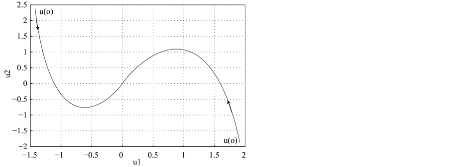
Figure 1.
Trajectories of the system
 from two different initial controls in
 .
.
negative real number, Theorem 5 ensures that all matrices F (row vectors) are of
the form KV where
 is a nonzero real solution to the simple “Sylvester equation”

This equation has a nonzero solution if, and only if, the real number
 is nonzero. That is,
 (17)
(17)
Formula
 shows that
 is a left eigenvector of
 associated to the undesirable eigenvalue
 and then
 for every
 . But pair
 is stabilizable, so

If we suppose that , then we should have

and then . We also have
 and
and . This shows that
 which is not true.
As a consequence, we have the following result.
Proposition 3 For a given left eigenvector
 of
of
 associated to the unique eigenvalue
 and for a negative real number
 , we have
 and matrix
 given by
 (18)
(18)
The spectrum of
 is then
 .
.
3.2. Case Where the Matrix VB Is Nonsingular
We have seen in the last paragraph that, when , a necessary and sufficient condition for Sylvester Equation
(15) to have nonsingular solution (nonzero real number in fact) is that the real
, a necessary and sufficient condition for Sylvester Equation
(15) to have nonsingular solution (nonzero real number in fact) is that the real
 is nonzero. We also have seen that this last condition;
 , is equivalent to the fact that pair
 is stabilizable. In case of
 , it may happen that pair
 is stabilizable but matrix
 is singular as will show the following example.
Example 2
Consider System (1) with

Eigenvalues of A are
 and
and . The last desirable eigenvalue
 is associated to the eigenvector
 of
of
 that spans the subspace
 . Matrix V is then

Matrix
 is singular since it is

Controllability matrix is given by

and is of full rank 3. This shows that pair
 is stabilizable since it is even controllable.
The case of matrix
 is nonsingular can be seen as a general case of
 when
when . So, it deserves a special study that will be the aim in the sequel
of this paragraph. In the following theorem, we give a necessary and sufficient
condition for matrix
. So, it deserves a special study that will be the aim in the sequel
of this paragraph. In the following theorem, we give a necessary and sufficient
condition for matrix
 to be nonsingular.
Theorem 6
Matrix
 is nonsingular if, and only if,
 and
and
 are complementary subspaces of
 ; that is,
 .
.
Proof.
The if part: Since VB is nonsingular, matrix B is of full rank m. To complete the
proof of the if part, we shall show that
 since the dimension of the subspace
 is n − m. Recall that VX = 0 for any vector X in
 . If now X is both in
 and Im(B), then there is
 such that X = BU and then

This shows that U = 0 since VB is nonsingular and, then, X = 0.
The only if part: From the fact that VX = 0 for any vector X in ; that is
 , V is of full rank m; that is
 . Moreover, from the fact that
 , we get

since V is linear. This shows that the rank of VB is m and that it is nonsingular.
The
following theorem gives another method to get a partial pole assignment under the
assumption that
 is nonsingular.
Theorem 7
Suppose that matrix
 is nonsingular and let matrix
 be such that
 ,
,
 and
and
 is nonsingular. Then,

where .
.
wang#title3_4:spwang#title3_4:spProof.
Let
 and
and . Then,

This shows that
 is a nonsingular solution to Sylvester Equation (16) and, by Theorem 5, that matrix
 satisfies
 ,
,
Example 3
Consider System (1) with

Eigenvalues of A are
 and
and . The last desirable eigenvalue
 is associated to the eigenvector
 of
of
 that spans the subspace
 . Matrix
 is then

Matrix
 is nonsingular and matrix
 is given by

Now choose
 that are the eigenvalues of the matrix
 . Then,

4. A Total Eigenstructure Problem
Note that, when m and n are equal, matrix V described in the last section is now
any invertible matrix of . That is why, we suppose
 . Then matrix
 is simply
 and Sylvester Equation (15) becomes
 (19)
(19)
where H is a real
 matrix with desirable spectrum. So, if the unique solution X of Equation (20) is
invertible, then the spectrum of
matrix with desirable spectrum. So, if the unique solution X of Equation (20) is
invertible, then the spectrum of
 and the one of H are equal, where matrix F is
 . Suppose now that
 . The technique of augmentation (see [5] and [6]
) consists of augmenting the matrix
. The technique of augmentation (see [5] and [6]
) consists of augmenting the matrix
 by adding zeros in order to get a new matrix
 . One should also complete the control vector
 by fictive real numbers to get
 . We also replace the assumption: “the pair
 is stabilizable” by “the pair
 is controllable.” System (1) which becomes
 (20)
(20)
does not change. The matrix
 is now a real
 matrix with some desirable spectrum
 which does not contain any eigenvalue of matrix
 . If the unique solution
 of Sylvester equation
 (21)
(21)
is invertible, we let . The matrices
 and
and
 have the same spectrum
 . If
. If
 is the matrix of the first
 rows of
 , then
 assigns the spectrum of
 to
to .
.
Example 4
Consider the problem of stabilization of the following double integrator system
 (22)
(22)
with

subject to the constraint . The matrix
 and the vector
 are respectively augmented to

such that
 where
where
 and
and
 are fictive positive real numbers. Let, for example,
 and
and
 to get the domain
 in the Example 1. We choose the matrix

for which the eigenvalues are
 and the inequality (13) is satisfied. Then, we solve the Sylvester equation (20)
and get
and the inequality (13) is satisfied. Then, we solve the Sylvester equation (20)
and get

The feedback matrix , which represents the first row of
 , is then

The spectrum of
 is then
 .
.
As in Figure 1 but in the state space, Figure 2 plots two trajectories in the state space starting from two different and admissible initial states and, thanks to the asymptotic stability of the system and the invariance positive property, shows the state convergence to the origin without leaving the domain imposed by the constraints.
5. Conclusion
A method for partial or total eigenstructure assignment problem was presented and
examples to illustrate the method were given. The method uses Sylvester equation
to find the feedback matrix F when some matrix
 is given with a desirable spectrum that will replace all the undesirable eigenvalues
of the initial matrix A of System (1) in the closed-loop. This method generalizes
the one proposed in [10] without additional conditions on Sys-
is given with a desirable spectrum that will replace all the undesirable eigenvalues
of the initial matrix A of System (1) in the closed-loop. This method generalizes
the one proposed in [10] without additional conditions on Sys-
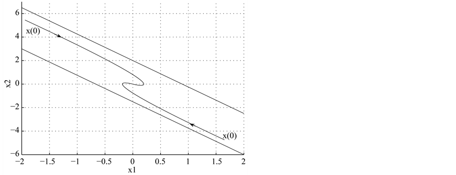
Figure 2. Trajectories
of the system
 from two different initial states
 such that
 .
.
tem (5) and allows us to deal with the problem of asymmetrical constraints on the control vector. Examples to show its importance are presented.
References
- Ait Rami, M., El Faiz, S., Benzaouia, A. and Tadeo, F. (2009) Robust Exact Pole Placement via an LMI-Based Algorithm. IEEE Transactions on Automatic Control, 54, 394-398. http://dx.doi.org/10.1109/TAC.2008.2008358
- Bachelier, O., Bosche, J. and Mehdi, D. (2006) On Pole Placement via Eigenstructure Assignment Approach. IEEE Transactions on Automatic Control, 51, 1554-1558. http://dx.doi.org/10.1109/TAC.2006.880809
- Sussmann, H.J., Sontag, E. and Yang, Y. (1994) A General Result on Stabilization of Linear Systems Using Bounded Control. IEEE Transactions on Automatic Control, 39, 2411-2424. http://dx.doi.org/10.1109/9.362853
- Benzaouia, A. (1994) The Resolution of the Equation
 and the Pole Assignment Problem. IEEE Transactions on Automatic Control, 40,
2091-2095. http://dx.doi.org/10.1109/9.328817
and the Pole Assignment Problem. IEEE Transactions on Automatic Control, 40,
2091-2095. http://dx.doi.org/10.1109/9.328817 - Benzaouia, A. and Burgat, C. (1988) Regulator Problem for Linear Discrete-Time Systems with Nonsymmetrical Constrained Control. International Journal of Control, 48, 2441-2451. http://dx.doi.org/10.1080/00207178808906339
- Benzaouia, A. and Hmamed, A. (1993) Regulator Problem for Linear Continuous-Time Systems with Nonsymmetrical Constrained Control. IEEE Transactions on Automatic Control, 38, 1556-1560. http://dx.doi.org/10.1109/9.241576
- Blanchini, F. (1999) Set Invariance in Control. Automatica, 35, 1747-1767. http://dx.doi.org/10.1016/S0005-1098(99)00113-2
- Gutman, P.O. and Hagander, P. (1985) A New Design of Constrained Controllers for Linear Systems. IEEE Transactions on Automatic Control, 30.
- Lu, J., Chiang, H. and Thorp, J.S. (1991) Partial Eigenstructure Assignment and Its Application to Large Scale Systems. IEEE Transactions on Automatic Control, 36.
- Baddou, A., Maarouf, H. and Benzaouia, A. (2013) Partial Eigenstructure Assignment Problem and Its Application to the Constrained Linear Problem. International Journal of Systems Science, 44, 908-915. http://dx.doi.org/10.1080/00207721.2011.649364
- Maarouf, H. and Baddou, A. (2012) An Eigenstructure Assignment Method, Publication and Oral Presentation at the International Symposium on Security and Safety of Complex Systems, Agadir.
- Barlaw, J.B., Manahem, M.M. and O’Leary, D.P. (1992) Constrained Matrix Sylvester Equations. SIAM Journal on Matrix Analysis and Applications, 13, 1-9. http://dx.doi.org/10.1137/0613002
- Ding, F. and Chen, T. (2005) Iterative Least-Squares Solutions of Coupled Sylvester Matrix Equations. Systems and Control Letters, 54, 95-107. http://dx.doi.org/10.1016/j.sysconle.2004.06.008
- Gardiner, J.D., Laub, A.J., Amato, J.J. and Moler, C.B. (1992) Solution to the Sylvester Matrix Equation AXBT + CXDT = E. ACM Transactions on Mathematical Software, 18, 223-231. http://dx.doi.org/10.1145/146847.146929
- Teran, F.D. and Dopico, F.M. (2011) Consistency and Efficient Solution of the Sylvester Equation for Congruence. International Linear Algebra Society, 22, 849-863.