Journal of Mathematical Finance
Vol.07 No.02(2017), Article ID:76693,22 pages
10.4236/jmf.2017.72024
A Stochastic Correlation Model with Time Change for Pricing Credit Spread Options
Zhigang Tong1,2, Allen Liu2
1Department of Mathematics and Statistics, University of Ottawa, Ottawa, Canada
2Model Validation, Enterprise Risk and Portfolio Management, Bank of Montreal, Toronto, Canada

Copyright © 2017 by authors and Scientific Research Publishing Inc.
This work is licensed under the Creative Commons Attribution International License (CC BY 4.0).
http://creativecommons.org/licenses/by/4.0/


Received: April 23, 2017; Accepted: May 28, 2017; Published: May 31, 2017
ABSTRACT
In this paper, we introduce the stochastic correlation processes for modeling the credit spread. We first model the components of spread process as correlated Ornstein-Uhlenbeck processes and correlation as Jacobi process. Using the properties of Jacobi process, we are able to obtain the analytical solutions for the credit spread option prices. To further enhance the model’s ability to capture the abrupt changes in the observed correlation time series, we construct a new model where the correlation is modeled by a Jacobi process time change by Lévy subordinators. We employ the eigenfunction expansion me- thods to obtain the closed-form solutions for the option prices. Our empirical study indicates the time changed Jacobi process fits the correlation series significantly better than the Jacobi process.
Keywords:
Stochastic Correlation, Jacobi Process, Stochastic Time Change, Eigenfunction Expansion, Credit Spread Options

1. Introduction
A credit spread option is an option on a particular borrower’s credit spread. The credit spread is the difference between the yield on the borrower’s debt and the yield on Treasury debt of the same maturity. The credit spread represents the risk premium that the market demands for holding the borrower’s debt. Unlike the credit default swaps, the payoff of credit spread options depends solely on the measurement of the credit spread rather than a specific credit event. Credit spread options protect the holder of the borrower’s debt from the loss of the rising yield spread due to default or credit rating downgrade.
Most of the models used in the pricing of credit spread options belong to the multi-factor models where state variables are modeled as correlated stochastic processes. [1] proposes a valuation model for pricing credit spread options by assuming that the risk-free interest rate and logarithm of the credit spread follow correlated mean reverting diffusion processes. [2] argues that the spread should be modeled using its two components instead of the spread itself and he extends [1] by assuming that the risk-free rate and the two components of credit spread follow correlated Ornstein-Uhlenbeck (OU) processes. [3] proposes a very general mean reverting process for the credit spread and two stochastic volatility processes, the square-root process and the OU process. The volatility process is assumed to be correlated with the spread process. There are many other examples that employ correlated processes for modeling the credit spread and pricing credit spread options, see e.g. [4] - [9] .
Although most of the models stress the role played by the correlation between state variables for pricing credit spread options, a common assumption is that the correlation is constant. There is a growing literature that documents that the correlation is far from being constant and it should be modeled as a random process, just like interest rate, stock price and volatility. [10] provides analytical properties of the correlation process and provides a new approach of modeling correlation as a stochastic process. [11] and [12] propose a modified Jacobi process to evaluate risk premium of the stochastic correlation and develop a series solution for pricing options under the correlation risk. [13] provides a closed-form approximation for pricing of several two-dimensional derivatives under the assumptions of stochastic correlation. [14] and [15] propose to generate the stochastic correlation process through the hyperbolic transformation of any mean-reverting process with positive and negative values.
In this paper, the main problem we are going to solve is how to model the credit spread and price the credit spread options with the stochastic correlation process. We stress that so far most of stochastic correlation models are developed for the equity and foreign exchange derivatives, where the underlying state variables are usually modeled as correlated geometric Brownian motions. To model the credit spread, we need to take the mean-reversion in the state variables into consideration. In particular, we model the components of the spread process as correlated OU processes and stochastic correlation as Jacobi process which guarantees the correlation between state variables is a bounded process. Using the properties of Jacobi process, we are able to derive the analytical formula for the moments of integrated correlation process required for calculating the credit spread options prices. From the data we employ for the empirical study, we observe that the correlation process changes abruptly and a diffusion model may not fully capture its dynamics. We therefore develop a time-changed model for correlation process where the Jacobi process is time changed by Lévy subordinators to yield state-dependent jumps. To the best of our knowledge, the time-changed Jacobi process (TC-Jacobi) has not been studied in the literature for modeling correlation. We notice that the TC-Jacobi process remains analytically tractable and the closed-form solutions for the credit spread options we derive under the Jacobi process require only minor changes. Our empirical results demonstrate that indeed the TC-Jacobi process improves the fit of correlation process significantly compared to the Jacobi process.
The structure of the paper is as follows. In Section 2, we introduce the credit spread model with constant correlation. In Section 3 we extend the constant correlation model to stochastic correlation model. Using the properties of Jacobi process, we derive the closed-form solutions for credit spread option prices. We introduce the time change to Jacobi process in Section 4 and demonstrate that the analytical formulas remain little changed by employing the eigenfunction expansion method. We compare the performance of Jacobi process with the time changed process using the correlation time series in Section 5. We also numerically study the implications on the derivatives for both processes.
2. A Credit Spread Model with Constant Correlation
Let denote a probability space with an information filtration ( ). We assume that under physical measure , the dynamics of the two yields included in the credit spread, denoted by and , follow the correlated OU processes. Thus,
(1)
(2)
and
(3)
where . and are two dependent Brownian motions with constant correlation coefficient .
To price the credit spread options, we need to work under the risk-neutral measure . We assume that under the measure , the stochastic processes of and are still correlated Ornstein-Uhlenbeck processes, but with different coefficients to highlight the risk premium. Therefore,
(4)
(5)
and
(6)
Under the above assumptions, we know that at time T, under the measure Q the vector has a bivariate normal distribution with mean and covariance matrix given by
(7)
where
(8)
(9)
(10)
and
(11)
Let denote the price of a call option on credit spread with strike price and maturity . The option price can be calculated from
(12)
where is included in to highlight that option price depends on the correlation coefficient . is the risk-free short rate and for simplicity, we assume it is a constant.
Since follows a bivariate normal distribution, we know that is a Gaussian process with mean and variance
(13)
It becomes straightforward to compute the call option prices. We summarize the result in the following proposition (see also [2] and [12] ).
Proposition 1. Assume the dynamics of and are given by (4), (5) and (6) then the option price can be calculated by
(14)
where . is the CDF of standard normal distribution.
3. Stochastic Correlation with Jacobi Process
3.1. Motivation for Stochastic Correlation Process
In this section, we extend the constant correlation model in Section 2 by modeling the correlation coefficient as a stochastic process. To motivate our model, we first take a look at the data we use in the empirical study. Our data contain daily rates for 10-year constant maturity Treasury bonds and Moody’s Aaa and Baa seasoned bond indices. The data cover the period January 2, 1996 to July 25, 2016, for a total of 5146 observations. In Figure 1, we plot the time series of three yields and it is clear that all of them display mean reversion. We also construct the time series of correlation by the following procedure (similar to [10] [14] and [15] ):
1) At time , we regress daily changes in the values of and on the values of and a day before for a time window :
(15)
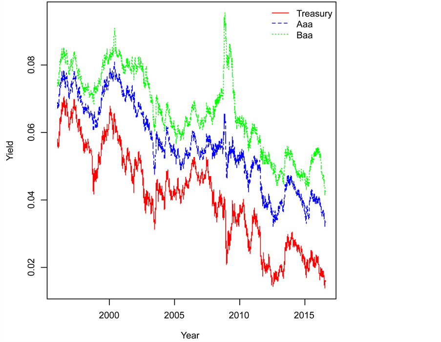
Figure 1. Time series of the yields of Treasury bonds and Moody’s Aaa and Baa seasoned bond indices.
and
(16)
2) The correlation is calculated by the correlation coefficient between and for a time window , that is
(17)
where and
We then roll over to time and so on to obtain a series of correlations through the time.
In Figure 2 we plot the dynamics of with . We can see clearly that the correlation is far from being constant and it varies very abruptly. The correlation is supposed to be bounded between −1 and 1, but in our dataset, it is concentrated on [0, 1]. In addition, the correlation process displays strong mean-reverting property. In Table 1, we provide the summary statistics for calculated from the two defaultable bond indices. The average correlations between the yields of Treasury bonds and Aaa and Baa bonds are around

Figure 2. Correlations between the yields for 10-year constant maturity Treasury bonds and Moody’s Aaa and Baa bond indices. Left panel: Aaa bond indices; right panel: Baa bond indices.

Table 1. Summary statistics of correlation series.
0.87, but the correlations fluctuate between 0.33 and 0.99. The density functions for the correlation series have negative skewness and fat tail.
To satisfy the properties of the correlation series displayed in our data, we model the correlation as a Jacobi process, which takes the value between and , i.e.
(18)
and
(19)
where , and . is a standard Brownian motion and independent of and in (1) and (2).
Under the martingale measure , we assume the stochastic process of is
(20)
where , and . is a standard Brownian motion under the measure and independent of and in (4) and (5).
The standard Jacobi process takes values between 0 and 1. Following [16] , we also impose the following conditions to ensure that the boundaries 0 and 1 are inaccessible to the process :
(21)
3.2. Properties of Jacobi Process
It is well known that there is no closed-form expression for the transition density for the Jacobi process (see e.g. [17] ). However, the transition density of Jacobi process can be represented in terms of eigenfunction expansions.
From (19), we know the infinitesimal generator of Jacobi process is
(22)
where is transformation function. and are first- and second-order derivatives of , respectively.
Let be the eigenvalues of and be the corresponding eigenfunctions, i.e.
(23)
We know for the Jacobi process defined on , the eigenvalues and eigenfunctions can be written as (see e.g. [16] and [17] )
(24)
and
(25)
where and
(26)
where , , . is the Jacobi polynomials defined as
(27)
where is the hypergeometric function defined by
(28)
The spectral decomposition allows us to find the transition density function of Jacobi process as
(29)
where is the stationary density function of Jacobi process ,
(30)
where is the Beta function defined by
(31)
where is the standard Gamma function.
The most important property of Jacobi polynomials is that they satisfy the following orthogonality condition (see e.g. [16] ):
Proposition 2.
(32)
Using this property, we can immediately have the following results:
Corollary 1. Let , and be nonnegative integers.
・ If , then
・ If , then
・ If , then
In this paper, we need to compute the following two integrals:
and
where and are two nonnegative integers.
We can prove the following results:
Lemma 1.
(i)
(33)
where
(34)
where is the hypergeometric function defined by
(35)
(ii)
(36)
where
(37)
Proof. To prove (i), from Corollary 1, we immediately know that for , the integral is clearly zero. For , we can use the following formula (see e.g. [18] ):
(38)
To prove (ii), we first use another representation of the Jacobi polynomials,
(39)
Then, we have
(40)
Using Corollary 1, we know that for , the above integral will be zero. If , we can compute the integral using the definition of function . □
In order to obtain the closed-form solution for the credit spread option prices, we are interested in computing the moments of the following integral
(41)
We can prove the following result:
Theorem 1.
(42)
where ,
(43)
, , and are assumed to be calculated using the coefficients under the measure .
Proof. First, we know
(44)
We have
(45)
Using the eigenfunction expansion for the transition density of Jacobi process , we have
(46)
For the first integral in the above equation,
(47)
For the second integral,
(48)
Using Lemma 1, we can see that if . Otherwise, we have
(49)
Finally, using the definition of , we obtain the final result. □
We are also interested in calculating the moments of the following quantity
(50)
Using binomial expansion, we immediately have
(51)
It is also easy to obtain the centered moments of from the uncentered moments. The general equation for converting the nth uncentered moment to the centered moment is
(52)
We provide the first two centered moments for as follows:
Corollary 2.
(53)
(54)
where
(55)
(56)
(57)
(58)
(59)
3.3. Credit Spread Option Prices under Jacobi Process
If is not a constant, but deterministic, the credit spread defined in Section 2 will still be a Gaussian process with same mean but different variance
(60)
where is defined in (50).
The pricing formula in (14) will be changed to
(61)
where .
If the correlation coefficient is a stochastic process, but independent of underlying processes for the two yields and , we can employ Taylor series expansion method to obtain the analytical formula for the spread credit spread option prices (see e.g. [11] [12] [13] )
(62)
where denotes the kth derivative of with respect to evaluated at the point .
In practice, we need to approximate the series using the first n terms to obtain the option prices
(63)
To estimate the truncation error, we use the remainder of Taylor’s formula. We know there exists such that
(64)
Then, the bound for the error of is
(65)
For example, the second-order approximation to the credit spread option price is
(66)
where and can be found from Corollary 2. The second- order derivative of is
(67)
4. Stochastic Correlation with Time Changed Jacobi Process
From Figure 2, it is clear that the correlation process changes abruptly through the time. We also know that the density function of correlation process has fat tail. These indicate that a diffusion process such as Jacobi process may not fully capture the main features of the correlation process and it is necessary to include the jumps into the correlation process. One way is to add the jump process directly into the correlation process in (19), which is the approach taken by [19] . The shortcoming of this approach is that it is difficult to ensure the correlation stays between and .
In this section, we model the correlation with Jacobi process time changed by Lévy subordinators to yield state-dependent jumps. The models with stochastic time changes have been studied in [20] and [21] for equity markets, [22] and [23] for credit markets and [24] and [25] for commodity markets. Here we model the stochastic correlation with time changed process.
4.1. Lévy Subordinator
A Lévy subordinator is a non-decreasing Lévy process with jumps and non-negative drift (see e.g. [26] ). The Laplace transform of a Lévy subordinator can be written as
(68)
where function is known as the Lévy exponent of the subordinator and is given by the Lévy-Khintchine formula (see e.g. [26] )
(69)
where is the drift term of . is the Lévy measure which must satisfy
(70)
An important sub-class of Lévy subordinators are the tempered stable subordinators. For such subordinators, the Lévy measure is given by
(71)
where and . Important special cases are the Gamma subordinator
with , the IG subordinator with and the compound Poisson sub-
ordinator with and . For such subordinators, the Lévy exponent is given by
(72)
4.2. The TC-Jacobi Process
We model the correlation as the TC-Jacobi process, i.e.
(73)
(74)
(75)
where is a Lévy subordinator and is a time-changed Jacobi process. Under the martingale measure , we assume the stochastic process of is
(76)
Therefore, the original Jacobi process is time changed by Lévy subordinator to generate jumps. With these specifications, the new correlation pro- cess is guaranteed to lie between and .
An important advantage of modeling the correlation as Jacobi process time changed by Lévy subordinator is that we can express the transition density of via eigenfunction expansion (see e.g. [24] and [25] ), i.e.
(77)
where , and are the eigenvalues, eigenfunctions and steady-state density of Jacobi process, respectively, which can be found in (24), (25) and (30). Thus, the eigenfunction expansion of remains the same form as , but with replaced by .
In order to obtain the closed-form solution for the credit spread option prices under the TC-Jacobi process, we need to calculate the moments of the following integral
(78)
Using the eigenfunction expansion of the transition density of , we see that
the moments of can be computed exactly same as
by replacing with . We immediately obtain the following result:
Theorem 2.
(79)
where
(80)
The credit spread options prices under the TC-Jacobi process can then be computed by employing exactly the same technique as Jacobi process.
5. Empirical Study and Numerical Analysis
5.1. Estimation of Stochastic Correlation
We estimate the Jacobi and TC-Jacobi processes using daily correlation series constructed as in Section 3. We choose maximum likelihood estimation (MLE) method for both models and the estimation is carried out by using R software. For a sample of size of the log conditional likelihood function is given by
(81)
where Θ is the set of parameters to be estimated. is the transition density function of . The transition density functions are
(82)
for Jacobi process and
(83)
for TC-Jacobi process.
The MLE approach based on eigenfunctions for Jacobi process has been investigated in [17] . They also compare the performance of MLE estimator with other estimators proposed in the literature, such as the estimator in [27] , which is a method of moments based on an approximation of score function or with a generalized method of moments (GMM) estimator. The MLE estimator is further compared with computer-intensive simulation-based estimator, such as the simulated method of moments (SMM). They show that MLE outperforms the other estimators relative to bias and variance, while being easy to implement.
In the estimation, we set and so that the correlation is bounded by 0 and 1. The estimation results are presented in Table 2. We notice that all the parameters for both Jacobi and TC-Jacobi processes are highly significant. For Jacobi process, the mean parameters are very close for the correlations calculated from Aaa and Baa bonds. The correlations for Aaa bonds have higher mean reversion and smaller variance compared to Baa bonds. Whence Lévy subordinator is included, we clearly see that mean reversion and variance parameters drop significantly. This is as expected since the time-change process introduces the mean-reverting jumps into the correlation process, which is contrary to Jacobi process where the only source to generate mean reversion is through diffusion process.
We also report the log-likelihood function values, Akaike Information Criterion (AIC) and the Bayes Information Criterion (BIC) in Table 2. It is clear for the correlation calculated from both Aaa and Baa bonds, the TC-Jacobi model produces much larger likelihood values than Jacobi model, which
Table 2. Estimation results for the correlation processes.
The standard errors are in the parentheses.
indicates that it is necessary to include the jumps into the Jacobi process to improve its performance. We also employ AIC and BIC to compare the relative performance of Jacobi and TC-Jacobi processes. Again, it is clear that TC-Jacobi process captures the dynamics of the correlation much better than the Jacobi process.
5.2. Numerical Analysis of Credit Spread Options
We compute the credit spread option prices using second-order approximation that is provided in sections 3 and 4. The higher-order approximation yields similar results.
First, we test if stochastic correlation leads to different credit spread option prices compared to the constant correlation case. For the Jacobi process, we take the parameters from those reported in Table 2 based on the Aaa bonds. From Figure 3, we observe when the correlation process starts from the value lower/higher than the long-run mean, the prices under constant correlation

Figure 3. Comparison of credit spread option prices between stochastic and constant correlation. Top panel: ; middle panel: ; bottom panel: . The parameters for correlation process are obtained from Table 2. and
will be higher/lower than those under the stochastic correlation. When starting value is close to the long-run mean, there is no decisive difference between the two prices. These are due to the fact that under the Jacobi process, the correlation will converge to the long-run mean due to the strong mean-reversion. When the correlation is higher, the variance of credit spread will be lower, which will lead to the lower option prices and vice versa.
Second, we test if there is significant difference in the prices from the Jacobi and TC-Jacobi processes. We use the parameters from those in Table 2 for Aaa bonds for both correlation processes. From Figure 4 it is clear the prices from the TC-Jacobi process are higher than those from Jacobi process. This can be explained by the fact that the long-run mean from the TC-Jacobi process is lower than the Jacobi process.
In Figure 5, we also illustrate the role of different parameters of TC-Jacobi process played in the pricing of credit spread options. We vary each parameter while keeping others at values reported in Table 2. It seems that higher mean reversion parameter κ will lead to higher prices. As expected, increase in long-run mean will decrease the option prices. We also note there is no

Figure 4. Comparison of credit spread option prices from Jacobi and TC-Jacobi processes. Left panel: ; right panel: . The parameters for correlation process are obtained from Table 2. and

Figure 5. Credit spread option prices with different parameters from TC-Jacobi process. The parameters for correlation process are obtained from Table 2. and
significant effect on the prices for different volatility parameters. Finally, we find the higher , the lower in the Lévy process, the higher the price is.
6. Conclusions
In this paper, we introduce the stochastic correlation process for modeling the credit spread. We model the components of spread process as correlated OU processes and correlation as Jacobi process. We study the properties of Jacobi process and show how to obtain the analytical solutions for credit spread options. To enhance the model’s ability to capture the main features of correlation process, we extend the Jacobi process to TC-Jacobi process where the correlation is modeled by a Jacobi process time changed by Lévy subordinators. We demonstrate that the TC-Jacobi process remains analytically tractable and the closed-form solutions for the credit spread options derived under the Jacobi process requires only minor changes. From an empirical study using the correlation series constructed from the yields on Treasury bonds and Aaa/Baa bonds, we demonstrate the superiority of TC-Jacobi compared to Jacobi process for modeling the correlation. We also numerically illustrate that modeling the correlation as a stochastic process will have an effect on the option prices compared to the constant correlation model. Furthermore, there are differences in option prices from Jacobi and TC-Jacobi processes.
To keep our model as parsimonious as possible, we assume that both risk-free short rate and volatility are constants. It will be an interesting extension to allow them to be stochastic. As long as the stochastic processes for the short rate and volatility are independent of correlation process, our method of obtaining the closed-form solutions for option prices will continue to work. We would also like to apply the TC-Jacobi process to the modeling of correlation in equity, foreign exchange and commodity markets.
Acknowledgements
Zhigang Tong would like to thank NSERC for partially funding this work. The opinions in this article are solely those of the authors and do not reflect the official opinion of Bank of Montreal.
Cite this paper
Tong, Z.G. and Liu, A. (2017) A Stochastic Correlation Model with Time Change for Pricing Credit Spread Options. Journal of Mathematical Finance, 7, 445-466. https://doi.org/10.4236/jmf.2017.72024
References
- 1. Longstaff, F.A. and Schwartz, E.S. (1995) Valuing Credit Derivatives. The Journal of Fixed Income, 5, 6-12. https://doi.org/10.3905/jfi.1995.408138
- 2. Mougeot, N. (2000) Credit Spread Specification and the Pricing of Spread Options. Unpublished, Ecole des HEC.
- 3. Tahani, N. (2004) Valuing Credit Derivatives Using Gaussian Quadrature: A Stochastic Volatility Framework. Journal of Futures Markets, 24, 3-35. https://doi.org/10.1002/fut.10111
- 4. Chu, C.C. and Kwok, Y.K. (2003) No-Arbitrage Approach to Pricing Credit Spread Derivatives. The Journal of Derivatives, 10, 51-64. https://doi.org/10.3905/jod.2003.319201
- 5. Giacometti, R. and Teocchi, M. (2005) On Pricing of Credit Spread Options. European Journal of Operational Research, 163, 52-64.
- 6. Tchuindjo, L. (2007) Pricing of Multi-Defaultable Bonds with a Two-Correlated-Factor Hull-White Model. Applied Mathematical Finance, 14, 19-39. https://doi.org/10.1080/13504860600658943
- 7. Tchuindjo, L. (2011) Closed-Form Solutions for Pricing Credit-Risky Bonds and Bond Options. Applied Mathematics and Computation, 217, 6133-6143.
- 8. Romo, J.M. (2014) Modeling Credit Spreads under Multifactor Stochastic Volatility. The Spanish Review of Financial Economics, 12, 40-45.
- 9. Chen, S.N., Hsu, P.P. and Li, C.Y. (2016) Pricing Credit-Risky Bonds and Spread Options Modelling Credit-Spread Term Structures with Two-Dimensional Markov-Modulated Jump-Diffusion. Quantitative Finance, 16, 573-592. https://doi.org/10.1080/14697688.2015.1058520
- 10. van Emmerich, C. (2006) Modelling Correlation as a Stochastic Process. Unpublished, University of Wuppertal, Wuppertal.
- 11. Ma, J. (2009) Pricing Foreign Equity Options with Stochastic Correlation and Volatility. Annals of Economics and Finance, 10, 303-327.
- 12. Ma, J. (2010) Multi-Factor Models for Pricing Correlation-Dependent Interest-Rate Contingent Claim. International Review of Applied Financial Issues and Economics, 2, 359-378.
- 13. Alvarez, A., Escobar, M. and Olivares, P. (2011) Pricing Two Dimensional Derivatives under Stochastic Correlation. International Journal of Financial Markets and Derivatives, 2, 265-287. https://doi.org/10.1504/IJFMD.2011.045598
- 14. Teng, L., Ehrhardt, M. and Günther, M. (2016) A Versatile Approach for Stochastic Correlation Using Hyperbolic Functions. International Journal of Computer Mathematics, 93, 524-539. https://doi.org/10.1080/00207160.2014.1002779
- 15. Teng, L., Ehrhardt, M. and Günther, M. (2016b) Modelling Stochastic Correlation. Journal of Mathematics in Industry, 6, 1-18.
- 16. Delbaen, F. and Shirakawa, H. (2002) An Interest Rate Model with Upper and Lower Bounds. Asia-Pacific Financial Markets, 9, 191-209. https://doi.org/10.1023/A:1024125430287
- 17. Valéry, P. and Gouriéroux, C. (2011) A Quasi-Likelihood Approach Based on Eigenfunctions for a Bounded-Valued Jacobi Process. Unpublished, HEC, Montréal.
- 18. Prudnikov, A.P., Brychkov, Y.A. and Marichev, O.I. (1986) Integrals and Series. Vol. 2, Gordon and Breach Science Publishers.
- 19. Zetocha, V. (2015) Jumping off the Bandwagon: Introducing Jumps to Equity Correlation. Unpublished, SSRN.
- 20. Carr, P., Geman, H., Madan, D.B. and Yor, M. (2003) Stochastic Volatility for Lévy Processes. Mathematical Finance, 13, 345-382. https://doi.org/10.1111/1467-9965.00020
- 21. Carr, P. and Wu L. (2004) Time Changed Lévy Processes and Option Pricing. Journal of Financial Economics, 71, 113-141.
- 22. Mendoza-Arriaga, R., Carr, P. and Linetsky, V. (2010) Time Changed Markov Processes in Unified Credit-Equity Modeling. Mathematical Finance, 20, 527-569. https://doi.org/10.1111/j.1467-9965.2010.00411.x
- 23. Mendoza-Arriaga, R. and Linetsky, V. (2013) Time-Changed CIR Default Intensities with Two-Sided Mean-Reverting Jumps. The Annals of Applied Probability, 24, 811-856. https://doi.org/10.1214/13-AAP936
- 24. Li, L. and Linetsky, V. (2014) Time-Changed Ornstein-Uhlenbeck Processes and Their Applications in Commodity Derivative Models. Mathematical Finance, 24, 289-330. https://doi.org/10.1111/mafi.12003
- 25. Li, L., Mendoza-Arriaga, R., Mo, Z. and Mitchell, D. (2016) Modelling Electricity Prices: A Time Change Approach. Quantitative Finance, 16, 1089-1109. https://doi.org/10.1080/14697688.2015.1125521
- 26. Sato, K. (1999) Lévy Processes and Infinitely Divisible Distribution. Cambridge, UK.
- 27. Kessler, M. and Sorensen, M. (1999) Estimating Equations Based on Eigenfunctions for a Discretely Observed Diffusion Process. Bernoulli, 5, 299-314. https://doi.org/10.2307/3318437