Journal of Mathematical Finance
Vol.2 No.1(2012), Article ID:17602,9 pages DOI:10.4236/jmf.2012.21012
Analytical Hierarchy Process and Goal Programming Approach for Asset Allocation
1Finance Department, School of Business and Management, University of Quebec, Montreal, Canada
2Business Development Bank of Canada, Montreal, Canada
3School of Commerce and Administration, Laurentian University, Sudbury, Canada
Email: sedzro.k@uqam.ca, Marouane.arif@bdc.ca, tassogbavi@laurentian.ca
Received September 27, 2011; revised November 29, 2011; accepted December 8, 2011
Keywords: Asset allocation; Goal programming; Analytic hierarchy process
ABSTRACT
Asset allocation in portfolio construction must simultaneously consider market conditions and investors’ specific preferences. Therefore, it is a multi-criteria decision that goes beyond the scope of the two-criteria, mean and variance of the portfolio returns, optimization method that traditionally prevails in the financial literature. This article suggests a procedure that makes integrated asset management possible, based on the Analytic Hierarchy Process combined with a mean variance and goal programming model. We illustrate this procedure with data from Canadian mutual funds over a total period of five years and three months, from September 2002 to November 2007. The results obtained are encouraging, as the portfolios constructed in this manner perform better than the S&P/TSX 60 index, which is the reference portfolio for the Canadian market.
1. Introduction
We apply the Analytic Hierarchy Process (AHP), combined with a mean variance optimization and goal programming model to allocate assets within a portfolio, considering both market conditions and investors’ preferences.
Asset allocation is one of the most deciding tasks that influence portfolio performance. Brinson, Hood and Beebower [1] and Brinson, Singer and Beebower [2] show that investment policy accounts for an average of 93.6% of overall return variations, whereas selectivity and market timing only contribute slightly. Ibboston and Kaplan [3] confirms these results. They observe that asset allocation explains 90% of the variability of mutual funds overtime, 40% of variations between funds, and an average of 100% of a fund’s returns.
To aid managers in this exercise of decisive importance for portfolio performance, Sharpe [4] suggests an integrated approach to asset allocation that considers both market conditions, and the investor’s goals and wealth. Figure 1 below illustrates the major steps of this asset allocation process.
Quadrant C1 represents the current capital market conditions. Certain techniques must be used (quadrant C2) to translate these market conditions into asset return predictions (quadrant C3).
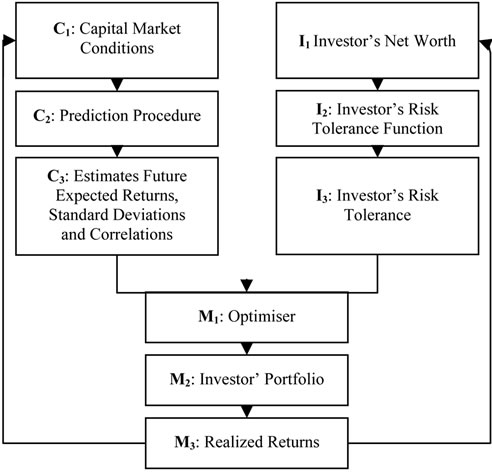
Figure 1. Integrated asset allocation. Adapted from [4].
The investor’s wealth (quadrant I1) usually determines his degree of risk tolerance (quadrant I3) through a risk tolerance function (quadrant I2).
Based on the degree of risk tolerance (quadrant I3) and asset return predictions (quadrant C3), an Optimizer (quadrant M1) can be used to determine the most suitable asset mix (quadrant M2) for the investor. Quadrant M3 represents the investor’s realized returns.
The returns for a given period will influence the value of the investor’s assets and liabilities at the beginning of the next period. Furthermore, the returns for a period will frame part of the market conditions at the beginning of the next period. Certain elements in quadrants C1, C3, I1, I3, M2, and M3 can change from one period to the next, whereas quadrants C2, I2 and M1 generally remain fixed.
Even though the overall integrated asset allocation approach can be considered relevant, there is no standard procedure for its implementation. For example, how can we account for the market conditions? Which model could we use to predict returns? How can we build a portfolio based on returns and the investor’s risk tolerance? All of these decisions remain specific to each manager or investor. In this regard, a survey conducted by Worzala and Bajtelsmit [5] shows vast variation in the decision-making process for big American pension funds managers.
In this article, we suggest a procedure based on the AHP put forward by Saaty [6] and goal programming model that can incorporate all factors deemed relevant to the asset allocation exercise. To make an analogy with the integrated asset allocation approach; 1) the AHP method makes it possible to consider both market conditions and investor preferences; 2) goal programming serves as an optimizer when building a portfolio that fits the investor’s goals.
The AHP is particularly appropriate when the decision to be made involves comparing elements that are subjective or difficult to quantify. In this case, it makes it possible to include all the factors that are judged relevant in the asset allocation process and that require choosing between: 1) different geographical area for international diversification purposes; 2) different asset classes (stocks, bonds, etc.); 3) different markets; 4) different securities. In addition, this method allows to develop a model that is easy to use and a fairly accurate representation of reality.
Therefore, first we apply the AHP method to determine the percentage of the portfolio to invest in each asset class based on economic scenarios and the investor’s risk profile. The AHP model’s outputs correspond to the proportions to invest in each asset class under consideration: stocks, bonds and liquid assets, based on analysts’ economic forecasts.
Second, we use a two-steps optimization procedure: 1) mean variance optimization to determine maximum return for the various levels of return variance; 2) The ratios obtained by running the AHP model are taken as goals for the goal optimization exercise, with constraints including the optimal returns and variances obtained during the first step.
We shall illustrate this two steps optimization procedure with data on returns and asset allocation for 77 mutual funds over a total period of five years and three months, from September 2002 to November 2007, a total of 63 months. Our application concerns an initial period of 36 months, namely from September 2005 to August 2007. Optimized portfolios determined in this manner are readjusted at the beginning of each following quarter, and returns are evaluated for the next quarter, for the following two years, namely from September 2002 to August 2004. For example, the first application deals with 36 monthly returns, namely from month 1 (September 2002) to month 36 (August 2005). The investment ratios obtained (for the end of August 2005 or for the beginning of September 2005) are applied to return 37, 38 and 39. The second application covers months 4 to 39 and returns are evaluated for months 40, 41 and 42, and so on through to month 63 (November 2007). The purpose is to determine the ex ante performance, that is the performance one would have achieved by using the suggested optimization process in the beginning of each quarter of this period.
The portfolios obtained show higher performance than the return for the SP/TSX60 index, the reference portfolio for the Canadian market.
We would like to point out that our suggested overall approach is likely to be useful to fund managers given its flexibility and ease of use. Furthermore, performance issues aside, it makes it possible to build a portfolio that suits the investor’s goals. In this respect, it can deflect lawsuits from swindled investors, like those faced by some American and Canadian brokers who advised their clients to build portfolios that did not match their investment goals.
The rest of this article is organized as follows: in Section II, we present the AHP methodology and the process for building portfolios. We discuss the goal optimization model in Section III. We will also illustrate the optimization process in that section, followed by a conclusion in Section IV.
2. The AHP Method
Developed by [6], the AHP is a technique used for dealing with complex, unstructured problems that involve the consideration of multiple criteria simultaneously. It is based on three principles: hierarchization, priority-setting and logical consistency [6].
• Hierarchization: this involves breaking down the problem into a homogenous set of components, and organizing them according to a hierarchy in order to incorporate significant quantities of information and present a more comprehensive portrait of the problem.
• Priority setting: this involves pairing elements at each level of the hierarchy by assigning a weight to each element as described in Table 1.
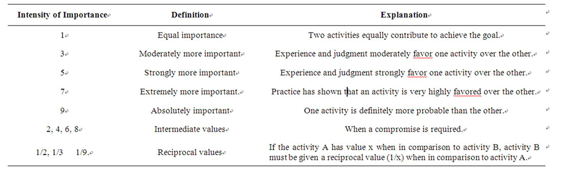
Table 1. The Analytic hierarchy process rating scales.
Source: adapted from [6].
• Logical consistency: since the various elements are paired using subjective means, such as judgment or opinion, the comparisons are not necessarily consistent. To remedy this, the AHP method uses a Consistency Index that enables to test the consistency of judgements systematically. For example: if A is considered five times preferable to B, and B is twice as preferable as C, than A must be considered 10 times preferable to C, otherwise the judgments are inconsistent.
2.1. Applying the Model
Applying the AHP approach involves first setting up the hierarchy of our decision-making process as shown in Figure 2 below. This hierarchy contains the factors that we find most relevant in the asset allocation process.
We begin by breaking down our main goal, namely,
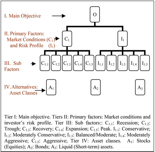
Figure 2. Hierarchy of the asset allocation decision process.
the proper allocation of assets, into two elements to which we grant equal importance: the investor’s risk profile (C1) and the state of the economy (C2).
Each of these two elements is subsequently broken down further into a set of five criteria: five risk profiles and five economic scenarios. Each investor must correspond to a risk profile, from C1.1 to C1.5 that can be determined, as in most financial institutions, using a questionnaire filled out by investors. To simplify, we assume that our investor’s risk profile remains the same (moderate) during the entire period of this study. The economic scenarios are based on economic predictions performed by Canadian banks and the Organization for Economic Cooperation and Development (OECD Thereafter). They reflect investors’ and financial service professionals’ expectations for each of the eight quarters considered in this study. These first three tiers of the hierarchy make it possible to determine the relative weight of each of the factors and criteria used. These weights vary overtime, except for the risk profile, which is assumed constant.
At the fourth and last level of the hierarchy, we find the various asset classes that make up the portfolio.
Once the hierarchy is established, we proceed with pairwise comparisons between elements at the various tiers of the hierarchy. The portfolio’s final composition will depend on the weight assigned to each element. These weights will constitute the inputs for our model, and can vary from one decision-maker to another depending on the importance granted to each of the factors considered.
Here are the comparison matrices that we explained in the next sections:
• Tier II: Risk profile and economic scenarios, a 2 × 2 matrix.
• Tier III: Criteria, a 5 × 5 matrix for economic scenarios. No analysis or matrix is needed for the investor profile, because we arbitrarily assume that it corresponds 100% to a moderate profile (C1.3).
• Tier IV: Asset classes, six 3 × 3 matrices.
2.2. Comparison of Tier II Elements
The two deciding factors in asset allocation are the investor’s risk profile and expected economic scenarios.
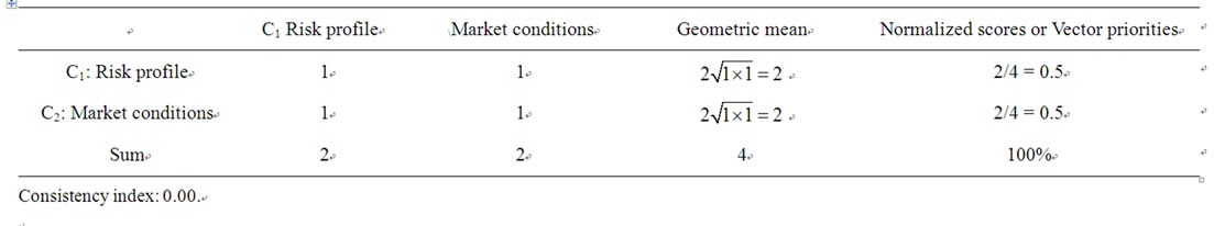
Table 2. Matrix for primary factor importance in the decision process (Tier II).
Consistency index: 0.00.
Table 2 shows the pairwise comparisons for these two elements respectively, and the method for calculating priorities or weights indicating the importance of particular criteria or alternative.
The number 1 implies that the investor’s risk profile is as important as economic scenarios when making asset allocation decisions.
The priority vector column in Table 2 shows the final ranking of factors based on their degree of importance. The 0.5 values assigned to C1 and C2 mean that these two elements are equally important.
This exercise must be performed from the top-down for factors at each tier of the hierarchy.
2.3. Comparison of Tier III Elements
We have classified economic scenarios according to their potential occurrence, drawing on the predictions of several Canadian banks and on the economic predictions of the OECD.

Table 3. Matrix for pairwise comparisons of economic scenarios (September 2005).
Consistency index: 0.02.
Table 3 shows the pairwise comparisons of economic scenarios as at September 1, 2005.
In the first column, the number 9 implies that a growth scenario is definitely more probable than a recession scenario. The number 7 implies that a peak scenario is very strongly more probable than a recession scenario. The resulted vector priorities may be interpreted as the predicted probability of the economy to be in a particular phase. For example, based on Table 3, one can say that there is 54.5% likelihood that the Canadian economy will be in the expansion phase in the quarter following September 2005 compare to 30.2% and 5.1%, 5.1% and 5.1% respectively for the peak, trough, recession, and recovery phases.
The comparison of economic scenarios is repeated for each of the following eight quarters. We summarize in Table 4,
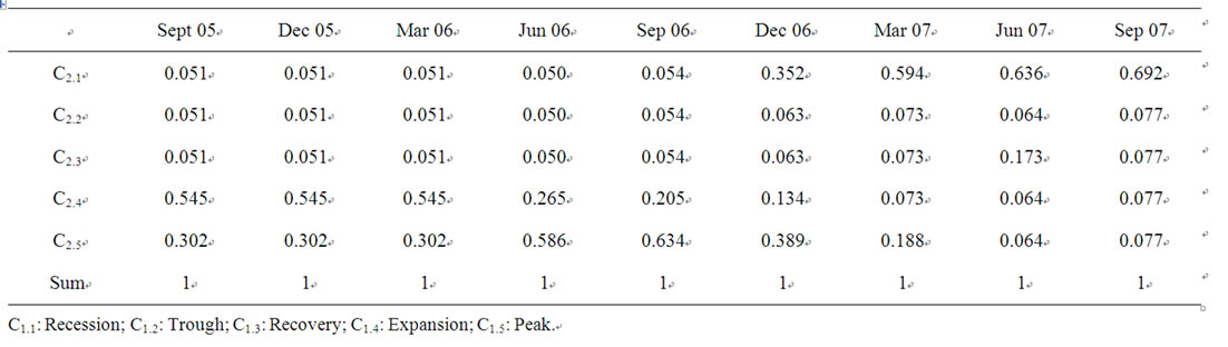
Table 4. Priority vectors resulting for comparison of economic scenarios for all the nine quarters of this study (September 2005 to September 2007).
the priority vectors resulting from this exercise for all the nine quarters of this study, September 2005 to November 2007. Detailed period from period results, as that of the September 2005 in Table 3, are available from the authors. One should note that the vector priorities in Table 4 must be adjusted for the importance of the factor of market conditions in our hierarchy. That is the result must be multiplied by 0.5 which is the weight assigned to the factor of market condition compare to the factor representing the investor risk profile.
2.4. Comparison of Level IV Elements
Here it is a matter of determining: 1) the behaviour of each asset class for each economic situation, as well as, 2) the asset classes in which it would be preferable to invest given the investor’s risk profile. In order to do this, we must ask the following question: “which asset class is it preferable to invest in given the two factors, economic situation and investor’s risk profile, in the third tier of the hierarchy?”
The answer to the first part of this question is provided in part in Table 5, built based on the findings of the studies Siegel [7] and Brocato and Steed [8], which suggest that each economic scenario favors investment in a specific asset class.
5: Over-weighting. i.e., increase the weight of these securities in the portfolio. 3: Neutral weighting. i.e., hold the weight of these securities in the portfolio. 1: Down-weighting. i.e., decrease the weight of these securities in the portfolio.
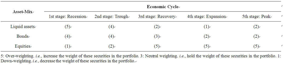
Table 5. Economic cycle and investment strategies.
Table 5 shows that during a recession, investment in short-term securities and bonds is highly preferred to investment in equities, which in turn are highly advisable in recovery, expansion and peak stages. Based on these results, Table 6 presents the pairwise comparisons of asset classes for the different economic scenarios.
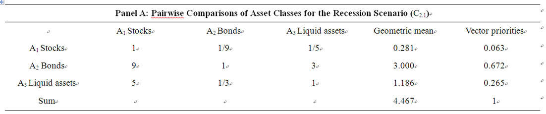
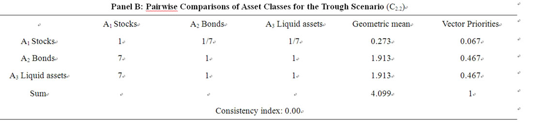

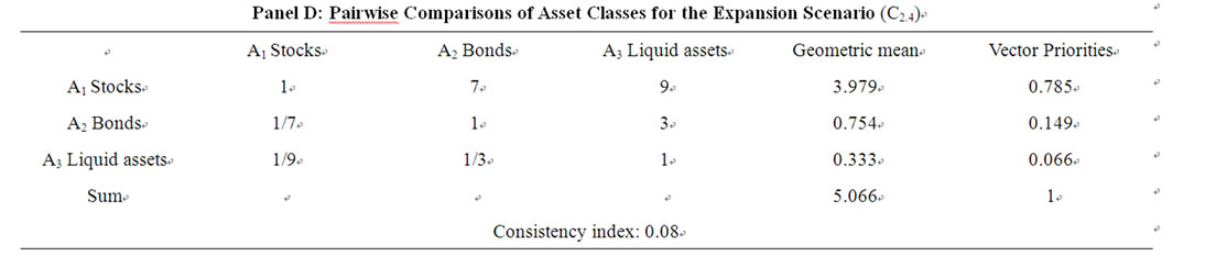
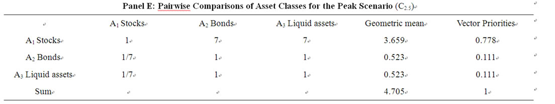
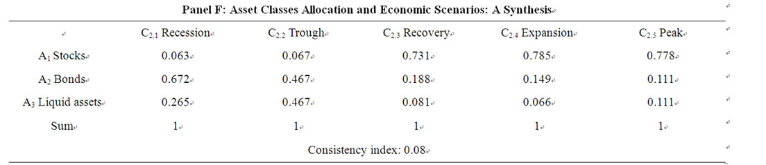
Table 6. Matrices of pairwise comparisons of asset classes for different economic scenarios.
For example, the number 9 (Panel A, first column) implies that, during a recession phase, investing in bonds is definitely preferable to investing in stocks. After performing the pairwise comparisons, we get the proportions to be invested in each asset class for each period by normalizing, as before, the geometric means of the score assigned to each alternative. We perform the same exercise for each of the four other economic scenarios: trough, recovery, expansion and peak, and the results are shown, respectively, in Panels B, C, D and E of Table 6. The results for all the five economic scenarios are summarised in the Panel F of the same Table.
As for the second part of the question, we consider only investor with a moderate risk profile.
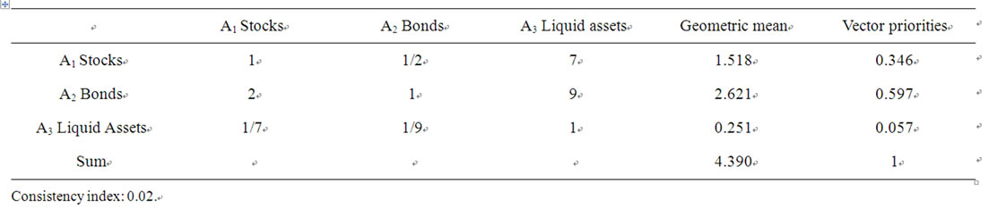
Table 7. Matrix of pairwise comparisons of asset classes for the balanced risk profile (C1.3).
Table 7 shows the resulting pairwise comparisons of asset classes where the number 2 implies that, for a person with a moderate risk profile, investing in bonds is slightly preferable to investing in stocks. Overall it is shown that a moderate risk profile investor will put 59,7% weight on bonds compare to 34.6% and 5.7% respectively on stocks and liquid assets or short term securities.
Finally, we have to weight the results of the asset classes allocation linked to economic scenarios (Table 6) and that related to investor risk profile (Table 7) against the priority assigned to the investor risk profile (Table 2) and the probability of occurrence of each economic scenario (Table 3). We then obtain the overall composite weight or investment ratios for each asset class for investor with a moderate risk profile and the predicted phase in the economic cycle. The result for September 2005 appears in Table 8" target="_self"> Table 8.
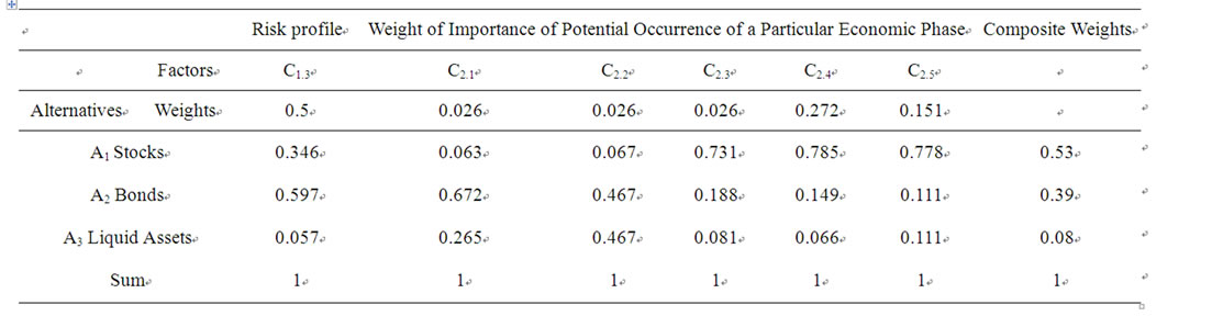
Table 8. Overall composite weight of the asset classes for investor with a moderate risk profile and the predicted phase in the economic cycle on September 2005. C2.1 recession C2.2 trough C2.3 recovery C2.4 expansion C2.5 peak.
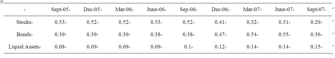
Table 9. Percentage of investment to be allocated in each asset class by an investor with a Moderate Risk Profile.
Table 9 synthesizes the investment ratios for each asset class for each of the nine periods of our study. These ratios change from one period to another due to change in the predicted economic scenarios. Indeed, as we have assumed that our particular investor will remain with a moderate risk profile, only the predicted economic scenario will affect the overall composite weight for each of the remaining periods in our study (Table 4).
These ratios are included as goals in the optimization model presented below to determine the optimal portfolio with a maximum return and a minimum risk.
3. Optimization Model
The weights obtained using the AHP are integrated into a two-steps optimization model. The initial purpose here is to determine the combination of funds that will produce maximum returns for a given level of risk.
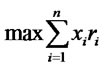 (1)
(1)
Subject to:
 (2)
(2)
 (3)
(3)
 (Impossibility of selling short) (4)
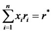
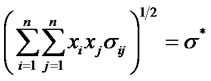
where ri represents the return of security i; xi = percentage of security i in the portfolio; n = total number of securities; sij = covariance of returns of security i in relation to security j. s = standard deviation of portfolio returns.
This classic Markowitz [9] model makes it possible to determine the optimal portfolio with maximum returns (r*) for a given standard deviation (s*). We shall recall that the optimal solution to this optimization problem is usually not unique. Therefore, the composition of this portfolio built according to optimal proportions, xi*, cannot respect our investor’s ideal goal about the proportion of stocks, bonds and liquid assets as determined using the AHP. To achieve this, we must proceed, as a second step, with goal optimization. The purpose here is to minimize deviations below the goal,  , and above the goal,
  , in relation to the ideal ratios of Stocks (S), Bonds (B) or Liquid Assets (L). Here is the formulation of the model:
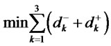 (5)
(5)
subject to:
 (6)
(6)
 (7)
(7)
 (8)
(8)
 (9)
(9)
 (10)
(10)
 (11)
(11)
 (12)
(12)
 (13)
(13)
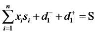
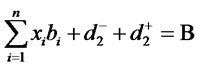
where ri, xi, n and sij are defined as above.  and
and  respectively represent deviations below and above the goal. r* represents maximum returns for a given standard deviation (s*). si, bi and li characterize the percentage of stocks, bonds or liquid assets in the fund i, respectively. S, B and L symbolize the proportion of stocks, bonds and liquid assets obtained using the AHP model.
The first two constraints make it possible to ensure that we maintain the level of return and standard deviation obtained during the first optimization. Constraints 10, 11 and 12 make it possible to ensure that the proportions of stocks, bonds and liquid assets are as close as possible to their ideal level (S, B and L).
4. Additional Data and Results
For illustration purposes, we have used monthly data on returns and asset distribution (stocks, bonds, liquid assets) for 77 mutual funds. This data comes from the Morningstar Canada database for the period from September 2002 to November 2007.
Optimization covers an initial period of 36 months, namely from September 2002 to August 2005, using the data for 77 mutual funds. In order to verify the ex ante efficiency of the optimization models, the obtained weights are multiplied by the returns for the next three months for the corresponding funds. For example, the first application covers 36 monthly returns, namely from month 1 (September 2002) to month 36 (August 2005). The investment ratios obtained (at the end of August 2005 or beginning of September 2005) are applied to returns for months 37, 38 and 39. The second application covers months 4 to 39 and returns are evaluated for months 40, 41 and 42. And so forth, up to month 63 (November 2007).
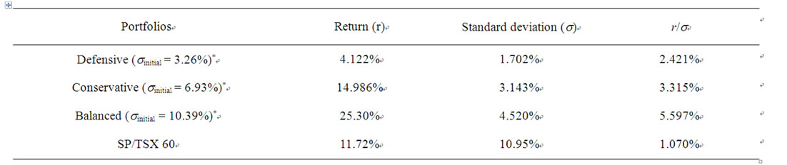
Table 10. Average annual realized returns (r) and Standard Deviations (s) obtained using the suggested optimization procedure from September 2005 to November 2007.
*sinitial is the initial (beginning of period) standard deviation of the portfolio.
Table 10 below summarizes the results obtained for three typical portfolios with monthly (annual) standard deviations preset at 1% (3.46%), 2% (6.93%) and 3% (10.39%).The portfolios obtained show better performance (returns by unit of risk) than the SP/TSX 60 index, the reference portfolio for the Canadian market.
In summary, we should mention that these illustrative tests show the flexibility and potential of the AHP approach combined with goal optimization models for portfolio allocation purpose. Here we have arbitrarily chosen three asset classes, but the method can accommodate several asset classes, for example, in the context of sector and geographic allocation.
5. Conclusions
In this study, we have illustrated the potential of the multicriteria AHP approach combined with a mean variance optimization and goal programming models when it comes to asset allocation that takes the investor’s risk profile and future economic scenarios as relevant elements. Our objective is to suggest a flexible approach that is relatively simple to use and that makes it possible to incorporate all factors, both objective and subjective, that are likely to influence the asset allocation decision. Our illustration draws on Sharpe’s integrated asset allocation model [4]. However, in the interest of simplicity, only three asset classes were considered (stocks, bonds and liquid assets). The selected criteria can vary from one manager to another, depending on his or her experience. In this respect, it is worth noting that the list of selected criteria is only presented as an example, and several other criteria can be added to or removed from the hierarchy, based on the manager’s judgment regarding their relevance.
As for future researches, it would be interesting to take the analysis further by proceeding with an industrial sector and geographic asset allocation. It might furthermore, be interesting to replace historical returns with predicted returns in the analysis.
REFERENCES
- G. P. Brinson, R. Hood and G. L. Beebower, “Determinants of Portfolio Performance,” Financial Analysts Journal, Vol. 42, No. 4, 1986, pp. 39-44. doi:10.2469/faj.v42.n4.39
- G. P. Brinson, B. D. Singer and G. L. Beebower, “Determinants of Portfolio Performance II: An Update,” Financial Analysts Journal, Vol. 47, No. 3, 1991, pp. 40-48. doi:10.2469/faj.v47.n3.40
- R. G. Ibboston and P. D. Kaplan, “Does Asset Allocation Policy Explain 40, 90, or 100 Percent of Performance?” Financial Analysts Journal, Vol. 56, No. 1, 2000, pp. 26- 33. doi:10.2469/faj.v56.n1.2327
- W. F. Sharpe, “Integrated Asset Allocation,” Financial Analysts Journal, Vol. 43, No. 5, 1987, pp. 25-32. doi:10.2469/faj.v43.n5.25
- E. M. Worzala and V. L. Bajtelsmit, “How Do Pension Fund Managers Really Make Asset Allocation Decision?” Benefits Quarterly, Vol. 15, No. 1, 1999, pp. 42-51.
- T. L. Saaty, “The Analytic Hierarchy Process,” McGrawHill Book Company, New York, 1980.
- J. J. Siegel, “Does It Pay Stock Investors to Forecast the Business Cycle?” Journal of Port-Folio Management, Vol. 18, No. 1, 1991, pp. 27-34. doi:10.3905/jpm.1991.27
- J. Brocato and S. Steed, “Optimal Asset Allocation Over the Business Cycle,” The Financial Review, Vol. 33, No. 3, 1998, pp. 129-148. doi:10.1111/j.1540-6288.1998.tb01387.x
- H. M. Markowitz, “Portfolio Selection: Efficient Diversification of Investments,” John Wiley & Sons, New York, 1959.