American Journal of Computational Mathematics
Vol. 2 No. 2 (2012) , Article ID: 20133 , 13 pages DOI:10.4236/ajcm.2012.22020
On the Coupled of NBEM and FEM for an Anisotropic Quasilinear Problem in Elongated Domains*
1School of Mathematical Science, Nanjing Normal University, Nanjing, China 2Jiangsu Provincial Key Laboratory for Numerical Simulation of Large Scale Complex Systems, Nanjing, China
Email: lyberal@163.com, duqikui@njnu.edu.cn
Received February 17, 2012; revised April 4, 2012; accepted April 14, 2012
Keywords: Quasilinear Elliptic Equation; Elliptic Artificial Boundary; Natural Integral Equation
ABSTRACT
In this paper, based on the Kirchhoff transformation, the coupling of natural boundary element method and finite element method are discussed for solving exterior anisotropic quasilinear problems with elliptic artificial boundary. By the principle of the natural boundary reduction, we obtain natural integral equation on elliptic artificial boundaries, the coupled variational problem and its numerical method. Moreover, the convergence and error estimate of the approximate solutions are obtained. Finally, some numerical examples are presented to illuminate the feasibility of the method.
1. Introduction
Based on the Green’s function and Green’s formula, natural boundary element method (NBEM) reduces the boundary value problem of partial differential equation into a hypersingular integral equation on the boundary, and then solves the latter numerically [1,2]. It has advantages over the usual boundary reduction methods: such as the diminution of the number of space dimensions by 1, the conservation of energy functional, the preservation of self-adjointness and coerciveness. But it also has evident limitations, it’s difficult to obtain Green’s functions for solving problem in general domains. Therefore, the coupling of NBEM which is also called artificial boundary condition [3,4] or DtN method [5,6] and finite element method (FEM) [2] is useful and necessary for general cases.
The standard procedure of the coupling method can be described as follows. We introduce an artificial boundary to divide the original domain into two subregions, a bounded inner region and an unbounded one with a special boundary, such as circle, ellipse, and spherical surface, on which the boundary element method and finite element method are used respectively. This technique has been used to solve many linear problems [1,2,4-6] and it has also been successfully generalized to solve nonlinear boundary value problems [7-9] or quasilinear problems [3,10,11]. The problems were discussed in [3,10,11] take circle as artificial boundary, but for the problems with elongated domains, an elliptic boundary that leads to a smaller computational domain is obviously better than the circle one. The purpose of the paper is to study the coupling of NBEM and FEM to solve the anisotropic quasilinear problems with an elliptic artificial boundary.
Let  be a elongated, bounded and simple connected domain in
  with sufficiently smooth boundary
 .
. . We consider the numerical solution of the exterior anisotropic quasilinear problem
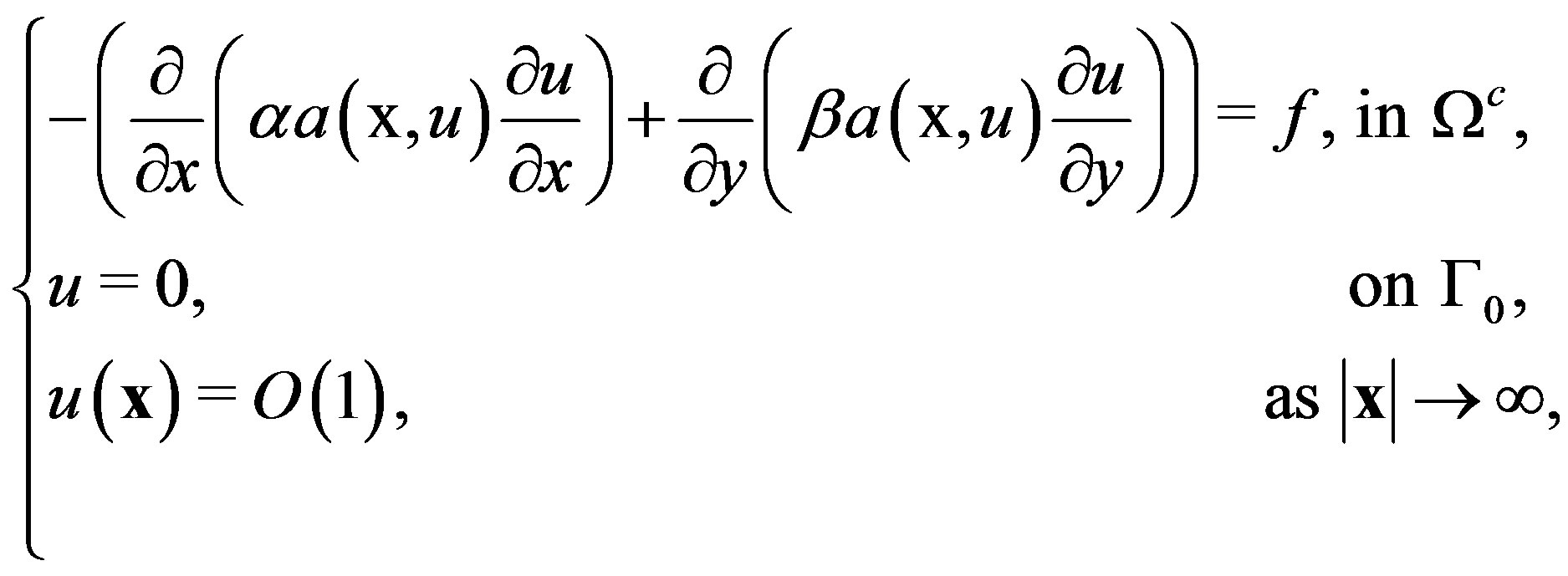 (1.1)
(1.1)
With  or
or ,
,  ,
,  and
and  are given functions which will be ranked as below. Following [3,12], suppose that the given function
  satisfies
 (1.2)
(1.2)
 where two positive constants
 , and
, and
 (1.3)
(1.3)
 with a constant
 . We also assume that
 ,
,  are continuous. In the following, we suppose that the function
  has compact support, i.e., there exists a constant
 , such that
 (1.4)
(1.4)
We also assume that
 (1.5)
(1.5)
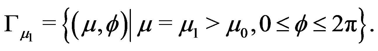
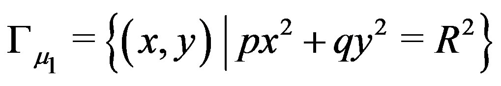
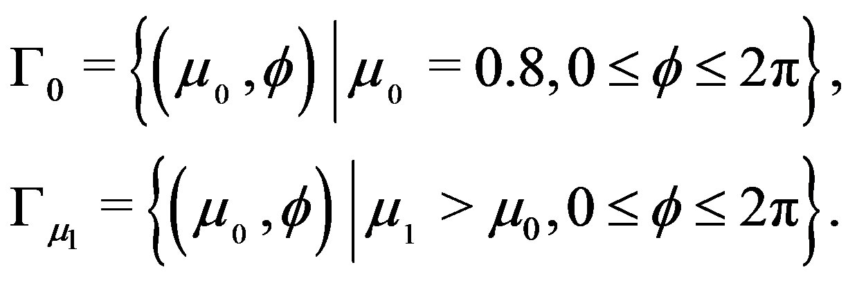
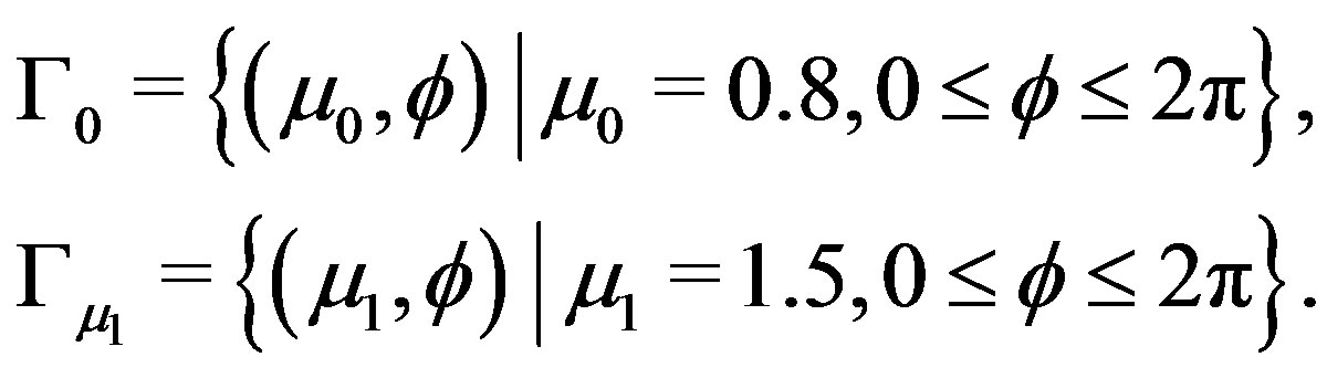
Now, we introduce an elliptic artificial boundary
 divide
  into two regions, a bounded domain
  and an unbounded domain
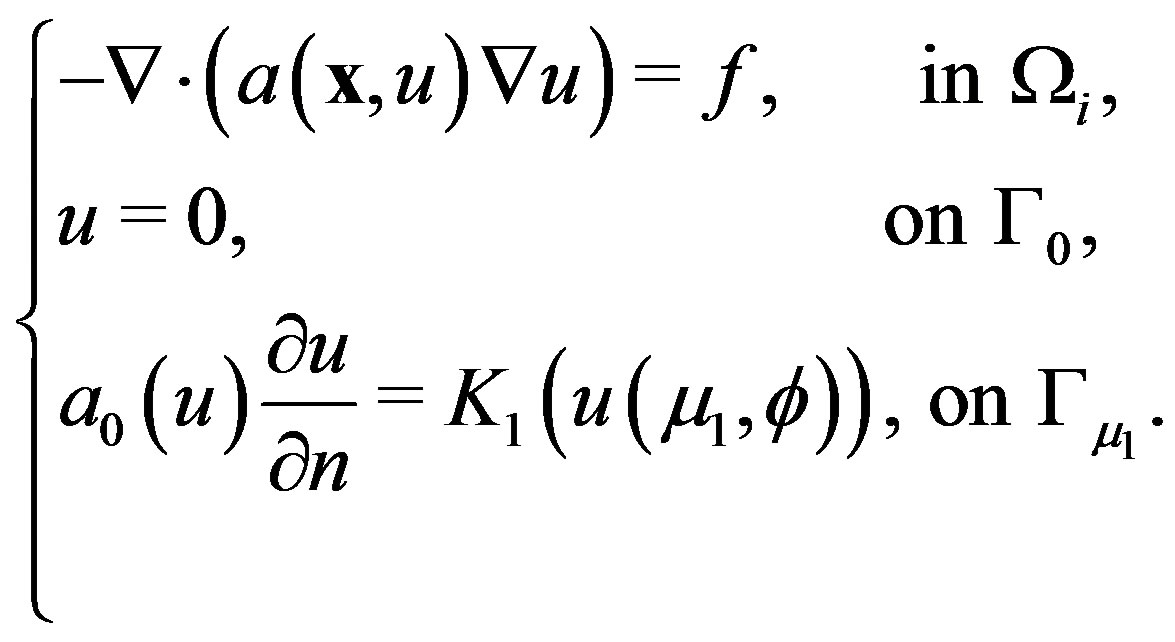
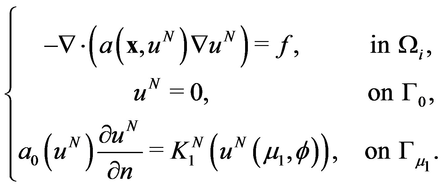
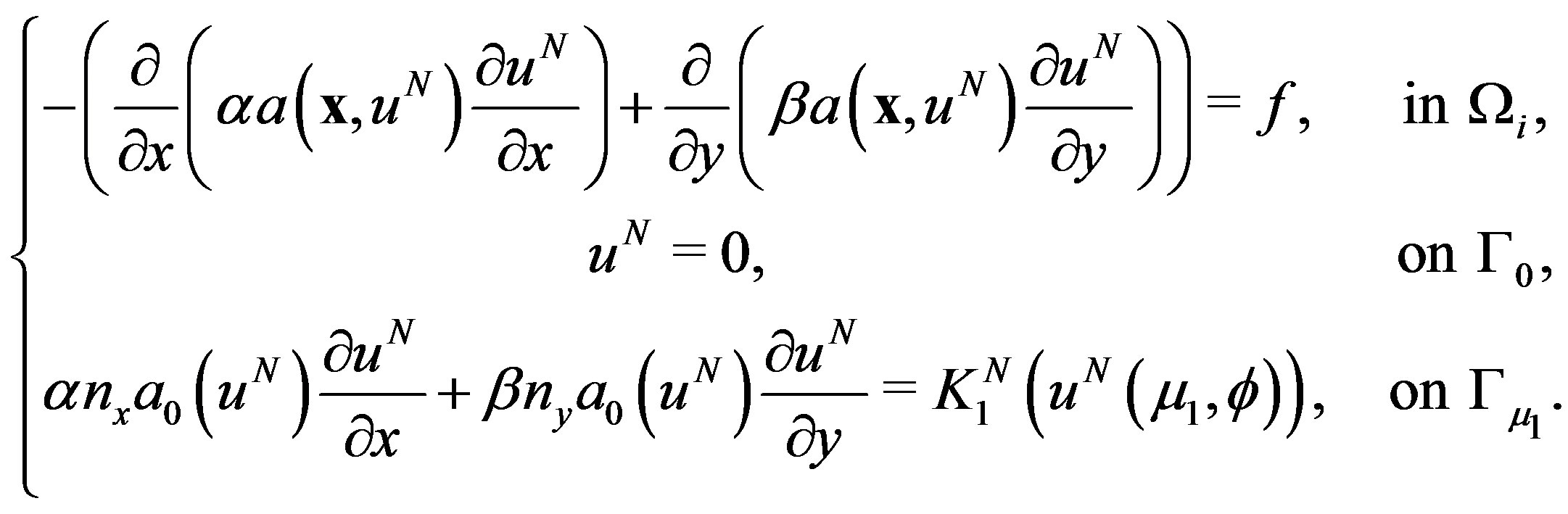
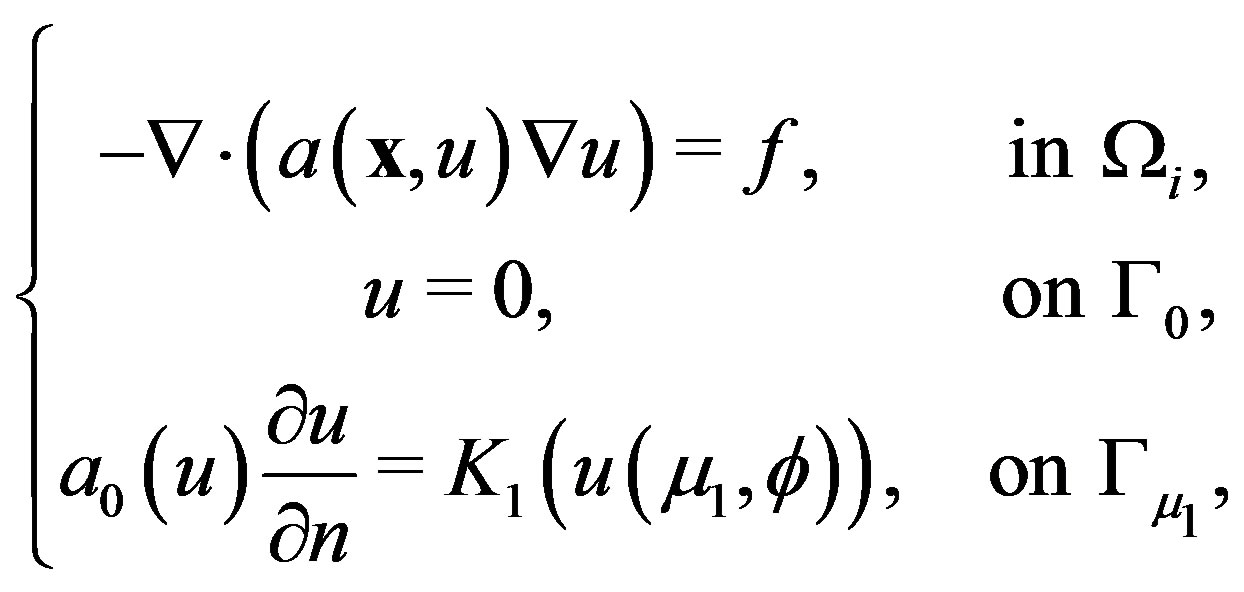
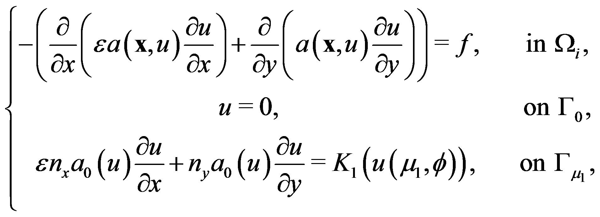
  with elliptic artificial boundary. Then the problem (1.1) can be rewritten in the coupled form:
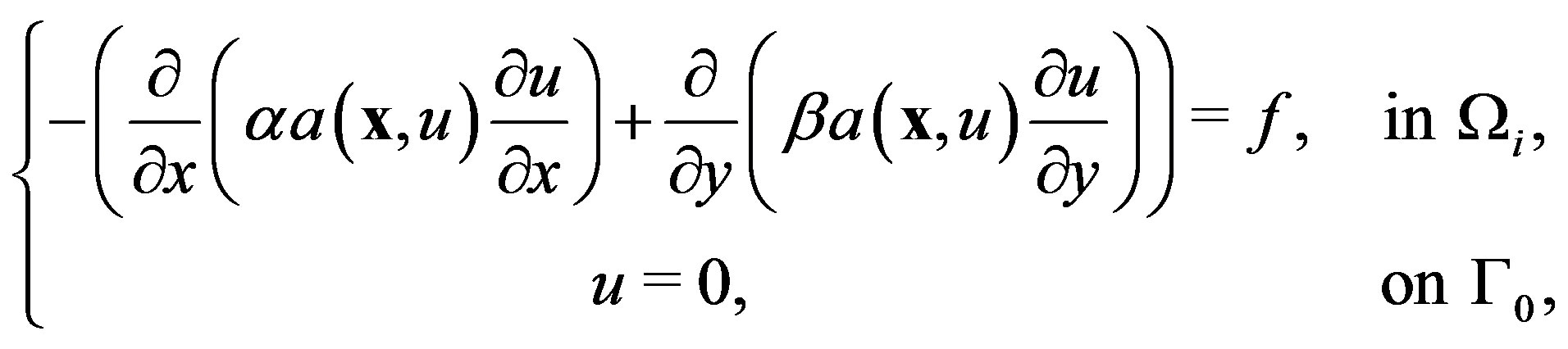 (1.6)
(1.6)
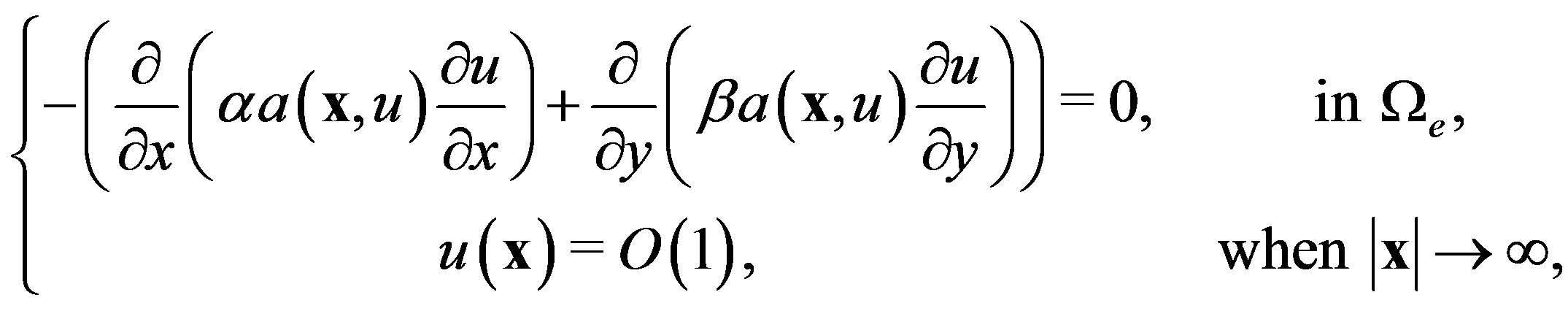 (1.7)
(1.7)
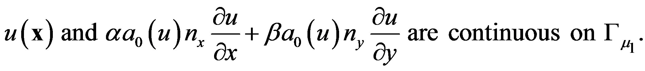 (1.8)
(1.8)
where  is the unit exterior normal vector on
 . Particularly, when
  which is independent of
  and
and , [13-15] have obtained the natural integral equation. We introduce the so-called Kirichhoff transformation [16]
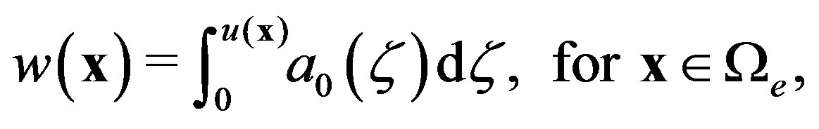 (1.9)
(1.9)
then we have
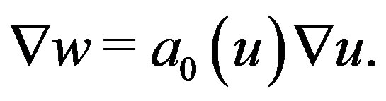 (1.10)
and
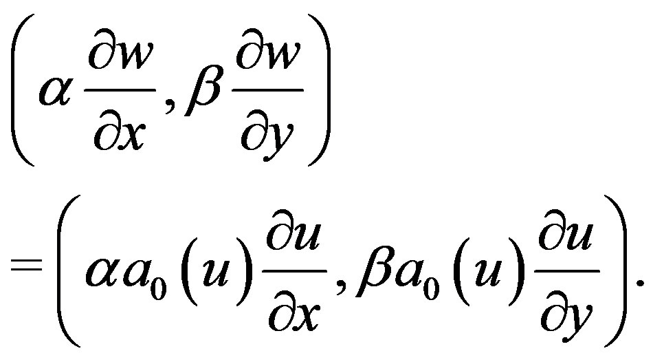 (1.11)
From equation (1.7) we have that  satisfies the following problem
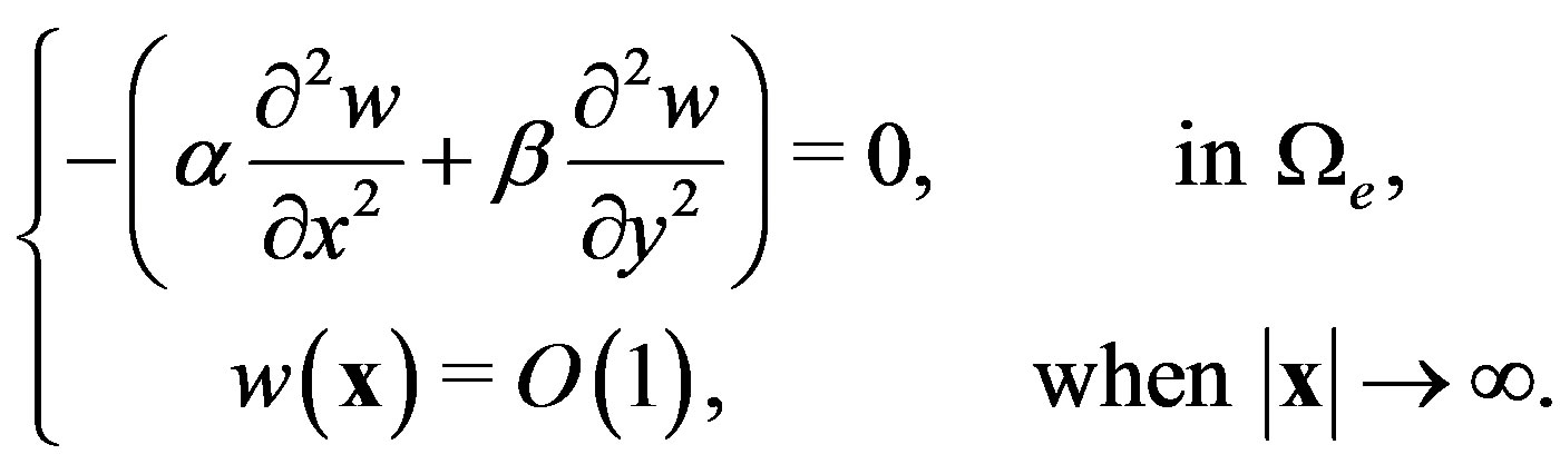 (1.12)
The rest of the paper is organized as follows. In section 2, we obtain the natural integral equation for elliptic unbounded domain cases. In section 3, we give the equivalent variational problems and the finite element approximations. The reduced problem’s well-posedness, the convergence results and error estimate are also discussed. At last, in section 4, we present some numerical examples to illuminate the efficiency and feasibility of our method.
2. Natural Boundary Reduction
In this section, by virtue of the Poisson integral formula and natural integral equation for the linear problem, we shall obtain the corresponding results for the quasilinear problem in . For this purpose, we need to discuss some properties between elliptic coordinates
  and Cartesian coordinates
  first. The relationship between the two coordinates can be expressed as below
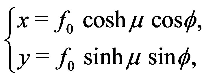 (2.1)
(2.1)
where ,
,  ,
, . Following from [15], we have
Theorem 2.1 The transformation between elliptic coordinates and Cartesian coordinates (2.1) possesses the following property.
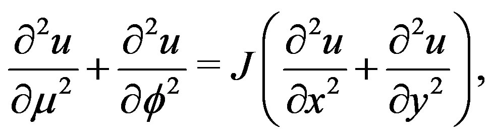
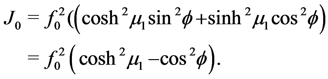
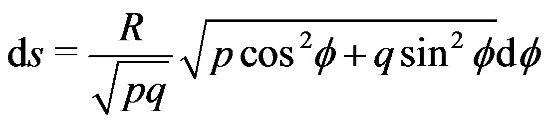
1) The Jacobi determinant of equation (2.1) is
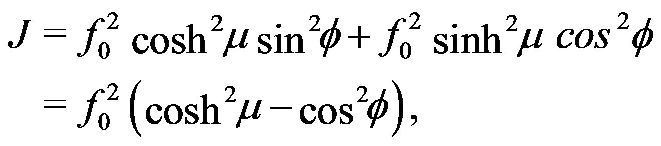 (2.2)
(2.2)
 if and only if
 ;
;
2)
 (2.3)
(2.3)
for ;
;
3) For the exterior domain 
 (2.4)
(2.4)
where  refers to the unit exterior normal vector on
  (regarded as the inner boundary of
 ).
).
Proof The conclusions 1 and 2 can be obtained by direct computation. And 3 follows from the property
2.1. Natural Integral Equation for α = β = 1
Assume that  is the solution of the problem (1.12), and the value
  is given, namely
Then based on the natural boundary reduction, there are the Poisson integral formulas
 (2.5)
(2.5)
or
 (2.6)
(2.6)
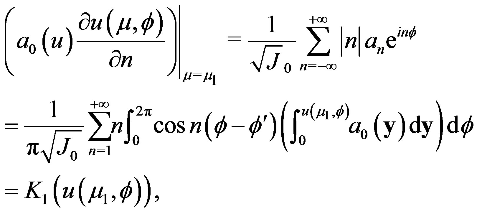
And the natural integral equation
 (2.7)
(2.7)
or
 (2.8)
(2.8)
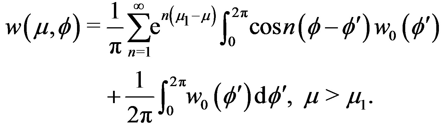
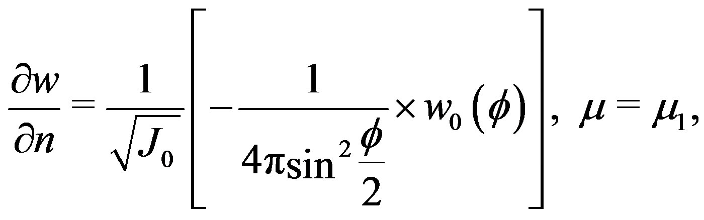
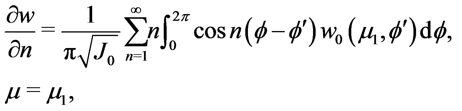
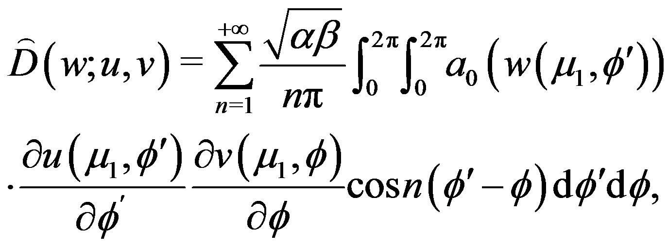
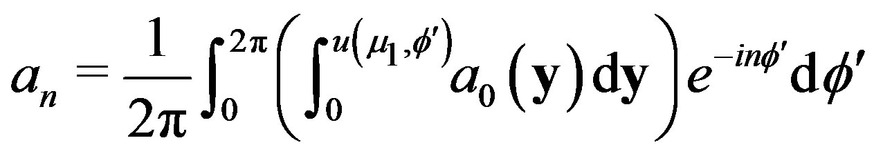
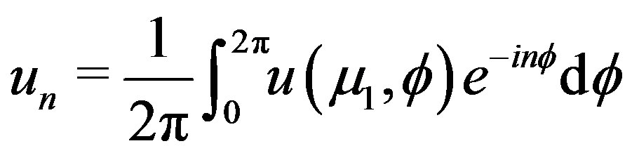
the definition of can be found in the following. The Poisson integral formulas (2.5) and (2.6) and the natural integral equations (2.7) and (2.8) can also be expressed in the Fourier series forms
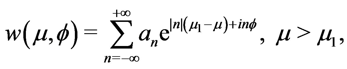 (2.9)
(2.9)
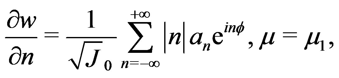 (2.10)
where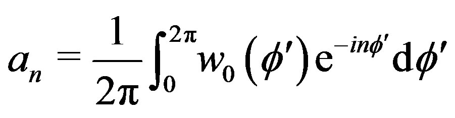 ,
,  and
and
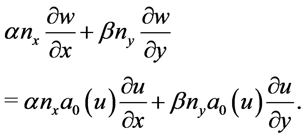
From (1.10), we obtain
 (2.11)
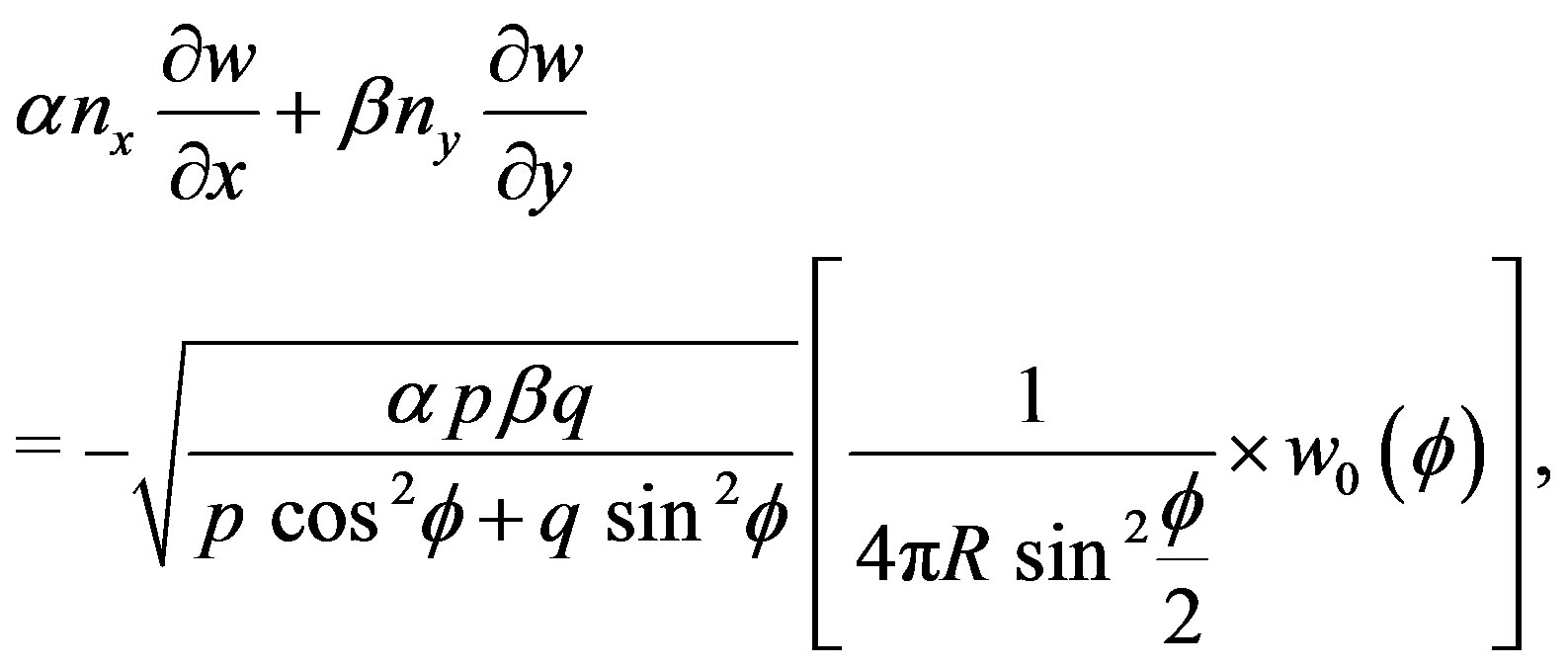
Combining (1.9), (2.10) and (2.11), we get the exact artificial boundary condition of  on
on ,
,
 (2.12)
where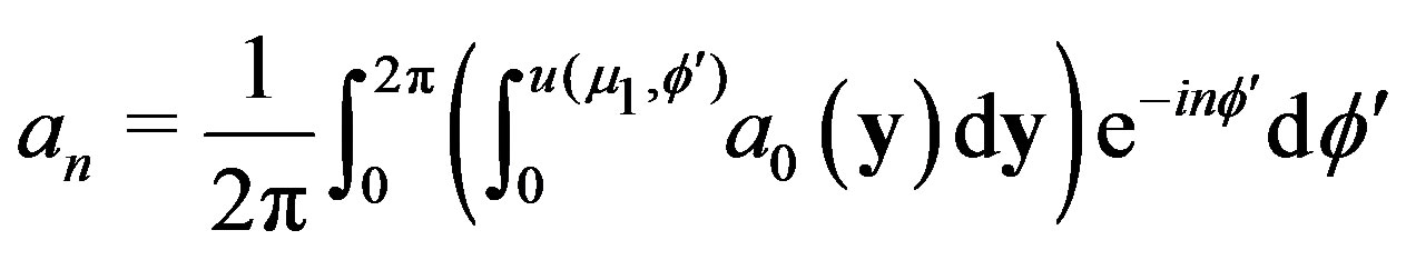 ,
,  ,
,
 . Then by (1.6)-(1.8) and (2.12), the original problem with
  confines in
  can be defined as follows
 (2.13)
Therefore, the solution of problem (2.13) is the solution of the problem (1.1) with  confining in the bounded domain
 .
.
2.2. Natural Integral Equation for β > α > 0
Now we assume that  can be expressed in the form:
 , with
 . We also assume that
  is the solution of the problem
(1.12), and the value  is given, namely

Let ,
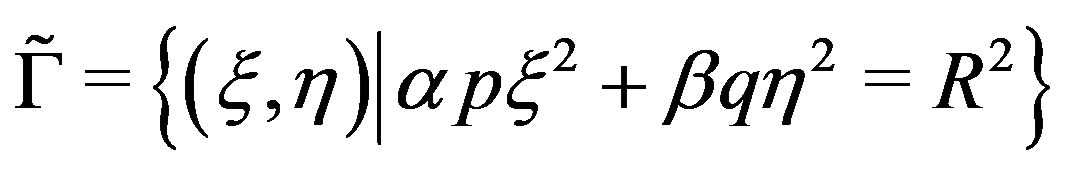
,  , then the boundary
  is changed by the elliptic boundary
 the unit exterior normal vector on
  is
is

By the above transformation, the problem (1.12) changes into
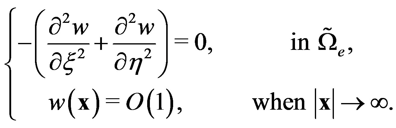 (2.14)
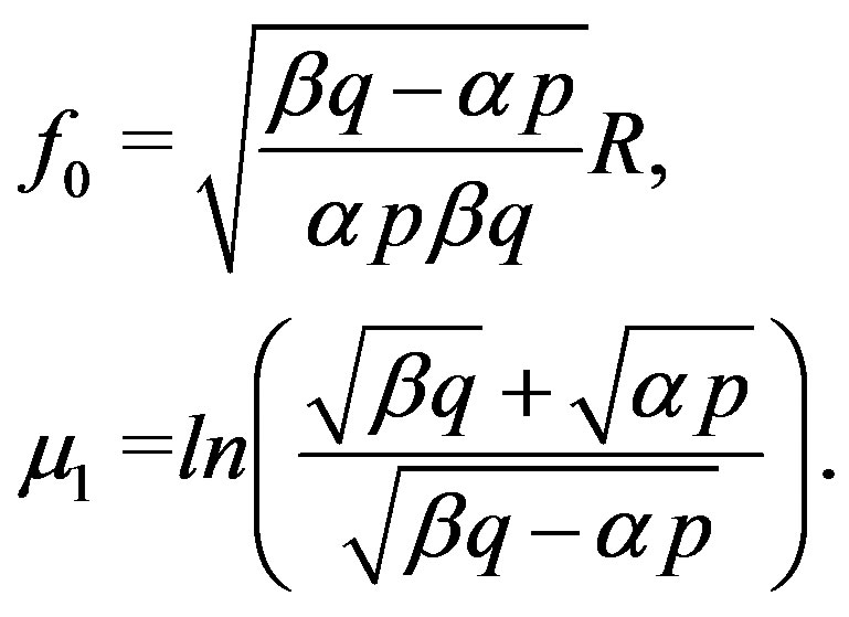
This is the right problem we talked in section 2.1. Similar with equation (2.1), we let

where
Then just the same as the problem discussed in Section 2.1, we have the natural integral equation on 
 (2.15)
where 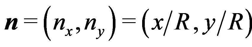 is the unit exterior normal vector on
 . From (1.11), we obtain
 (2.16)
Combining (1.9), (2.15) and (2.16), we obtain the exact artificial boundary condition of  on
on ,
,
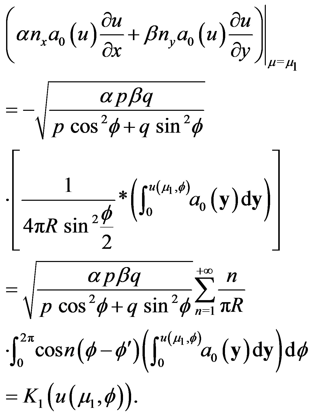 (2.17)
Then by (1.6)-(1.8) and (2.17), the original problem with  confines in
  can be defined as follows
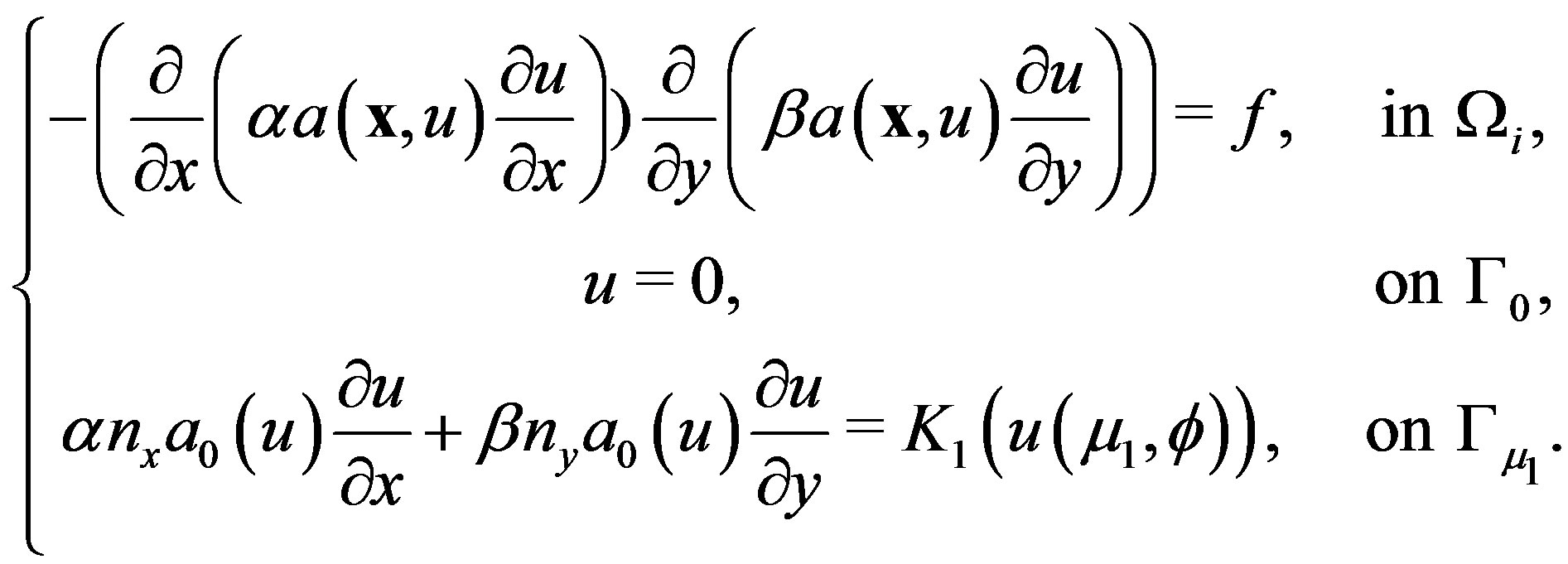 (2.18)
Therefore, the solution of problem (2.18) is the solution of the problem (1.1) with  confining in the bounded domain
 .
.
3. Variational Problem and Finite Element Approximation
3.1. The Equivalent Variational Problems
Now we consider the problems (2.13) and (2.18). We shall use  denoting the standard Sobolev spaces,
  and
and  referring to the corresponding norms and semi-norms. Especially, we define
 ,
,  and
and . Let us introduce the space
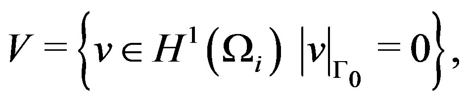 (3.1)
(3.1)
and the corresponding norms
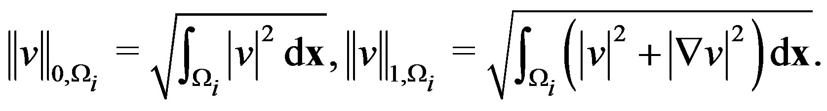
The boundary value problems (2.13) and (2.18) are equivalent to the following variational problem
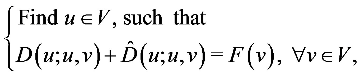 (3.2)
(3.2)
where
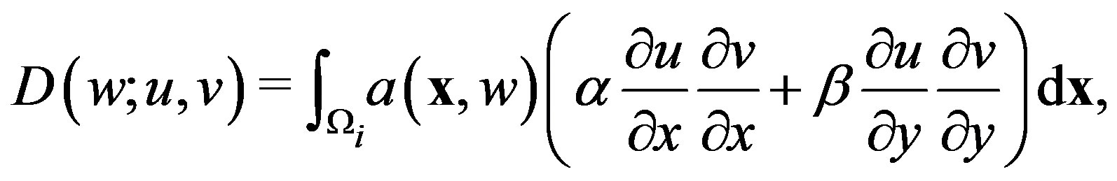 (3.3)
(3.3)
 (3.4)
(3.4)
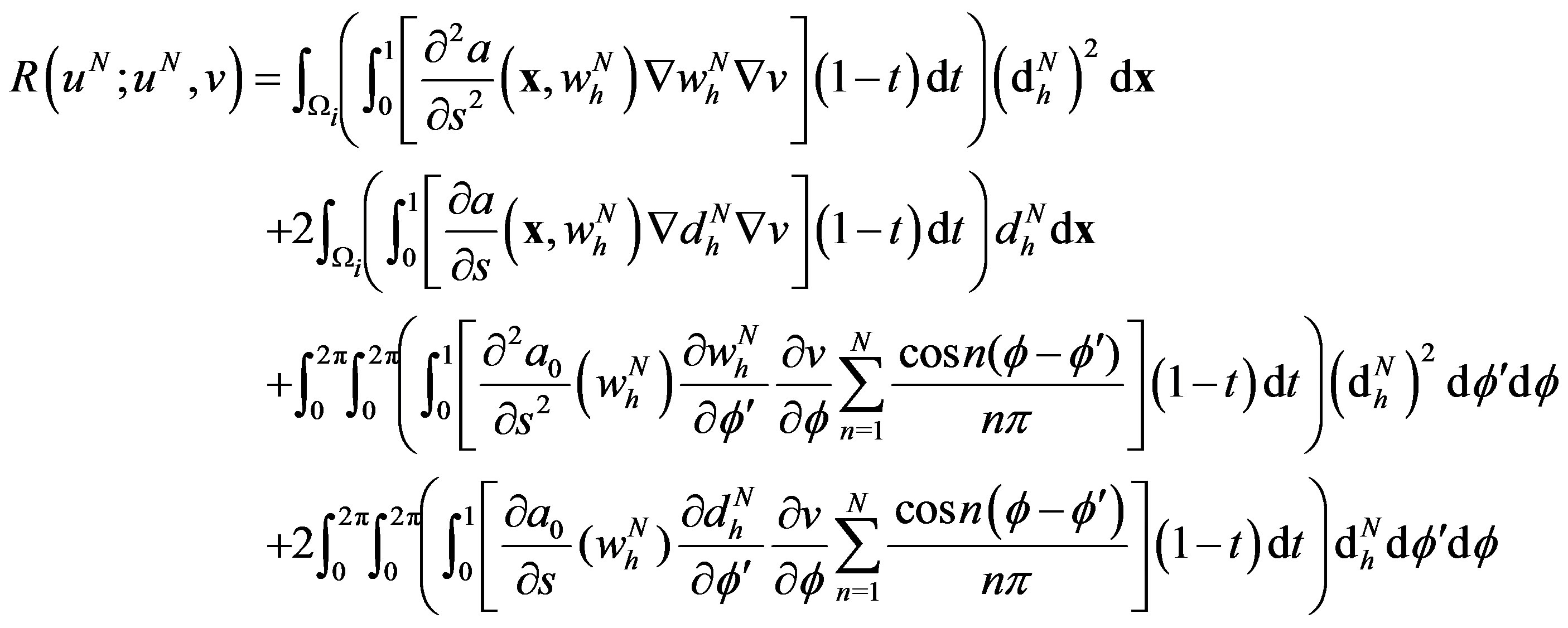
where  is gotten from Green’s formula, (2.7) and (2.8) with
 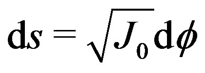 and (2.17) with
 .
.
 (3.5)
(3.5)
For any real number , we let
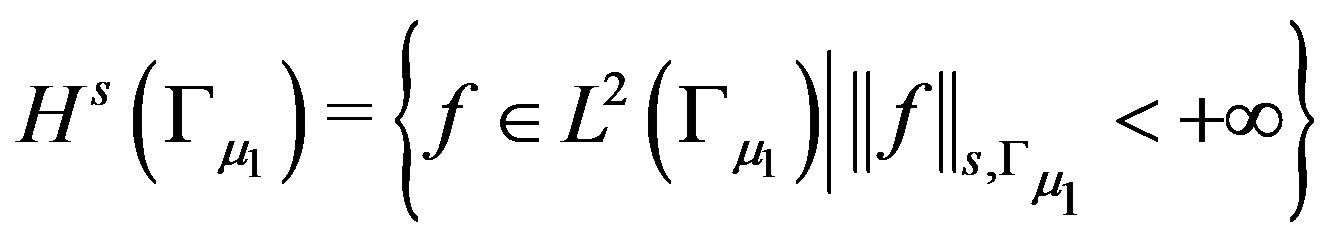 (3.6)
(3.6)
with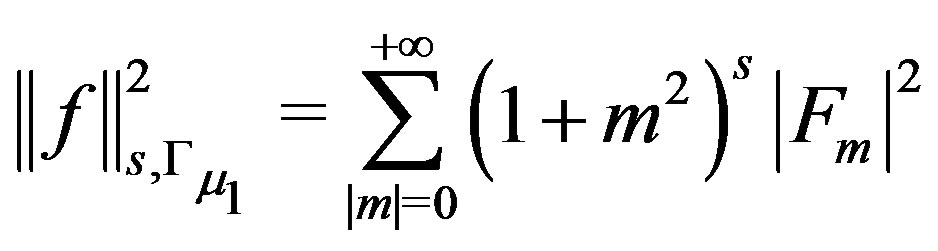 and
and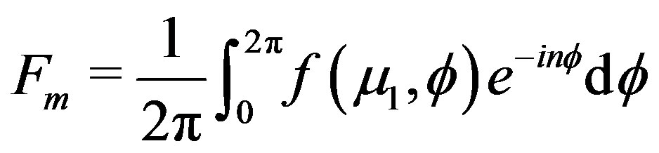 ,
, .
.
Lemma 3.1 There exists a constant  which has different meaning in different place and is related to
  and
and , such that
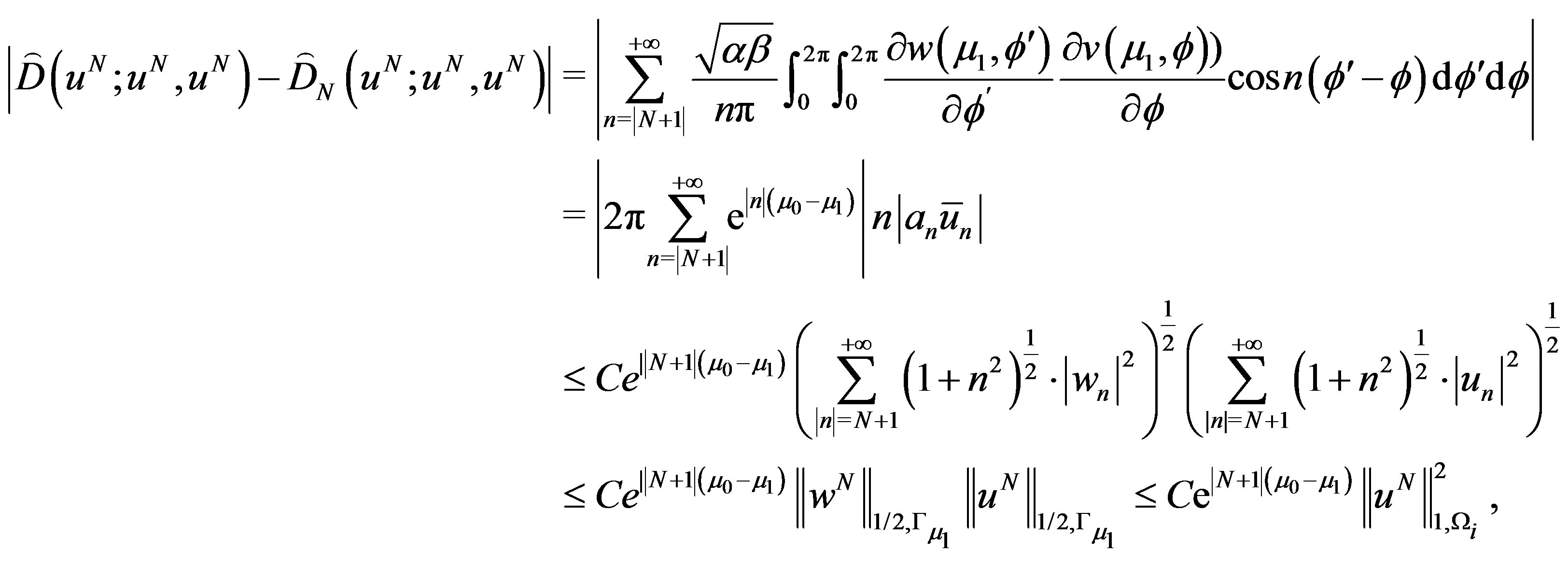
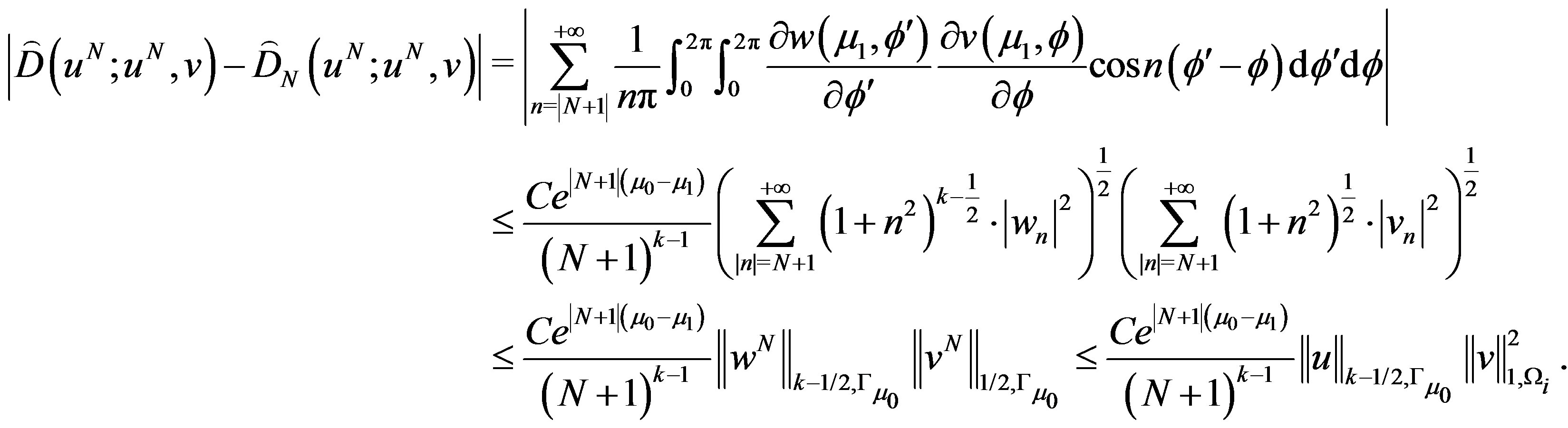
In practice, we need to truncate the series in (2.12) and (2.17) for some nonnegative integer , that is
 (3.7)
(3.7)
with
 (3.8)
(3.8)
when , and
, and
 (3.9)
(3.9)
when . So we only use the summation of the first
  terms in (2.13) and (2.18). We will consider the following approximate problem
 (3.10)
 (3.11)
Both (3.10) and (3.11) are equivalent to the following variational problem
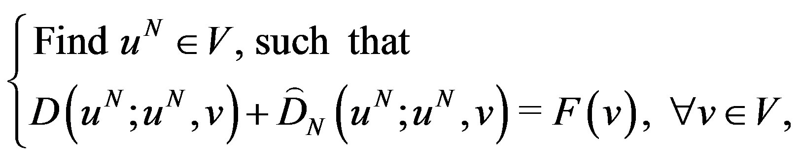 (3.12)
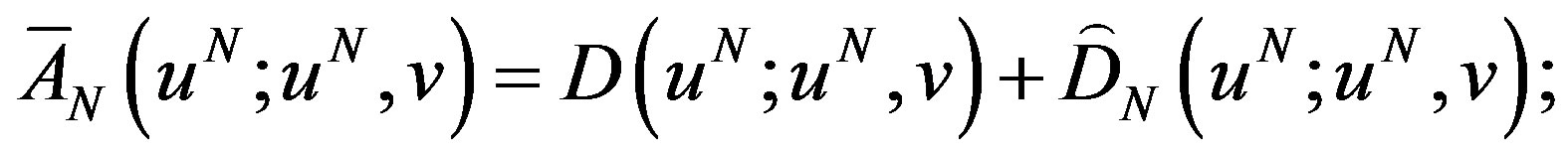
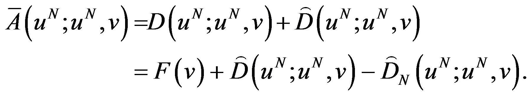
where
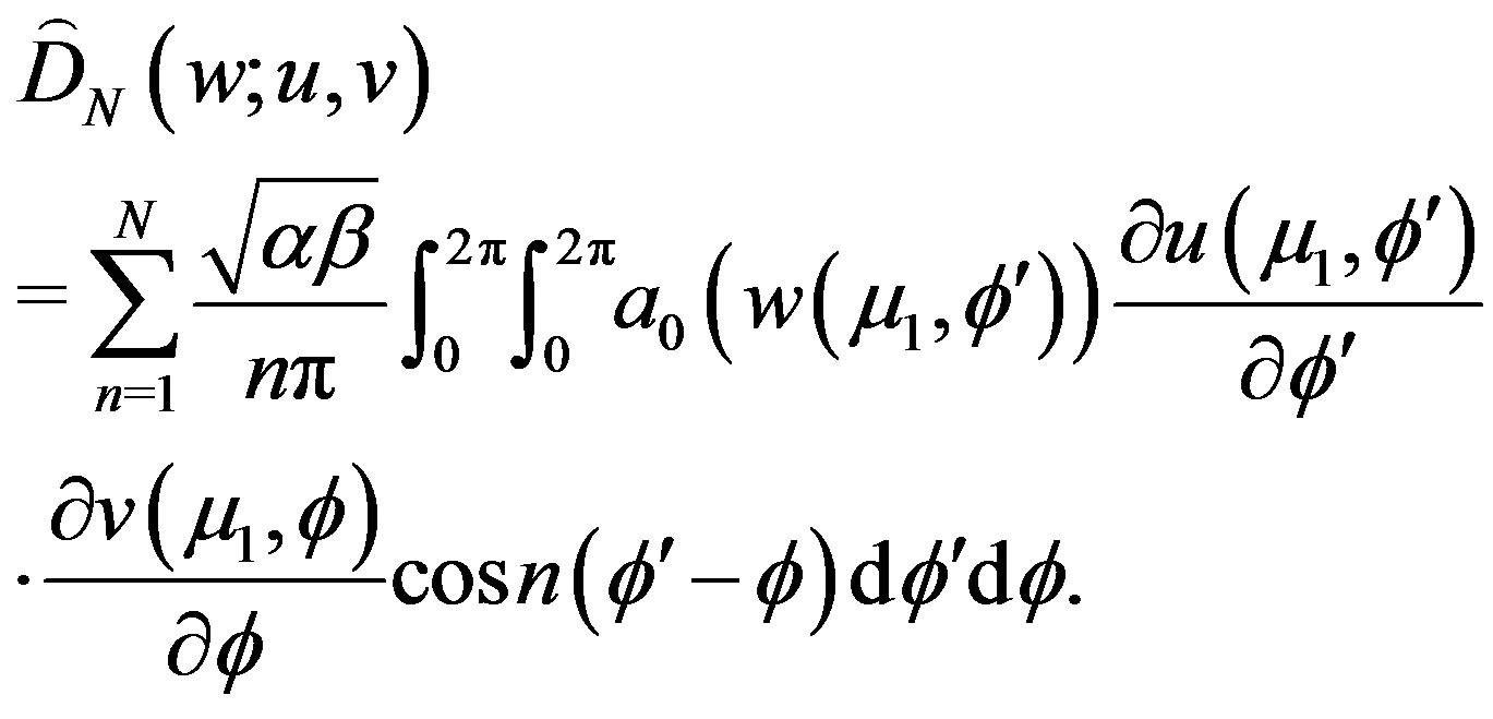 (3.13)
Similar with Lemma 3.1, we have
Lemma 3.2 There exists a constant  which has different meaning in different place, such that
3.2. Finite Element Approximation
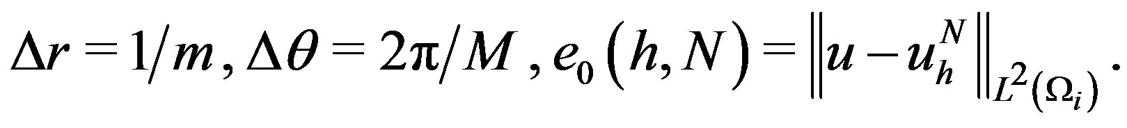
Divide the arc  into
into  parts and take a finite element subdivision in
  such that their nodes on
  are coincident. That is, we make a regular and quasiuniform triangulation
  on
on , such that
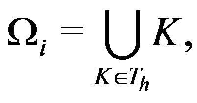 (3.14)
with  is a (curved) triangle;
  the maximum side of the triangles. Let
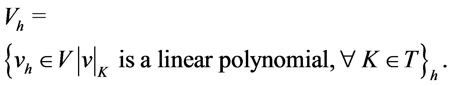 (3.15)
Then the approximate problem of (3.12) can be written as
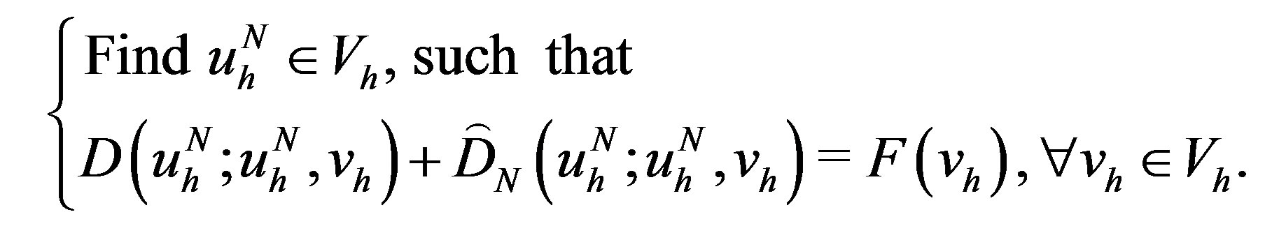 (3.16)
Some existence and uniqueness results for this type of problem are given in [12,17,18] under some conditions on the coefficients , so by the constraint conditions
(1.2) and (1.3) we have Lemma 3.3 Problems (3.2), (3.12) and (3.16) have unique solvability.
3.2.1. Convergence Theorems
In this section, we obtain the convergence result of the problems discussed above. We let  and
and  be the solution of problems (3.2), (3.12), (3.16) respectively. We also assume that
 (3.17)
And we require that  is a family of finitedimensional subspaces of
 , which satisfies for any
 (3.18)
 (3.19)
where  is independent of
 .
.
The continuous piecewise polynomial spaces, such as (3.15), satisfy the condition (3.17). And if we let
 , where
  is the interpolation operator, then by (3.19), we have

And we can also obtain the following result.
Lemma 3.4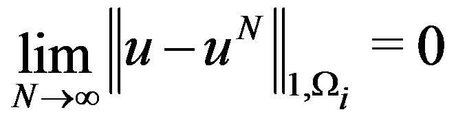 .
.
Proof From the (1.2), (3.12) and Lemma 3.2, we have
For , we assume that
with
 and
and
 .
.
Then we have
From , we obtain that
  is bounded in
 . Therefore, there exists a subsequence
  such that
 . Then similar with the proof of Lemma 3.4 of [3], we obtain
By the above lemmas, we get the following convergence result.
Theorem 3.1 Let , and the assumptions (3.17)-( 3.19) be satisfied, then we have
 (3.20)
3.2.2. Error Analysis
In the following, we shall get error estimates for the approximate solution obtained from a FEM-NBEM discrete scheme in the cases . We assume that the solution
  of problem (1.1) satisfies

For simplicity let us define the following notation

Then (3.2), (3.12), (3.16) can be replaced by the corresponding simple forms respectively.
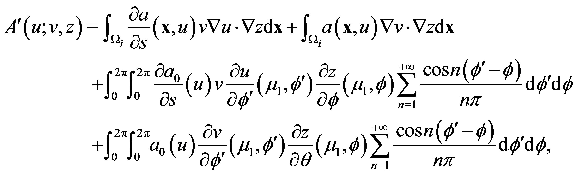
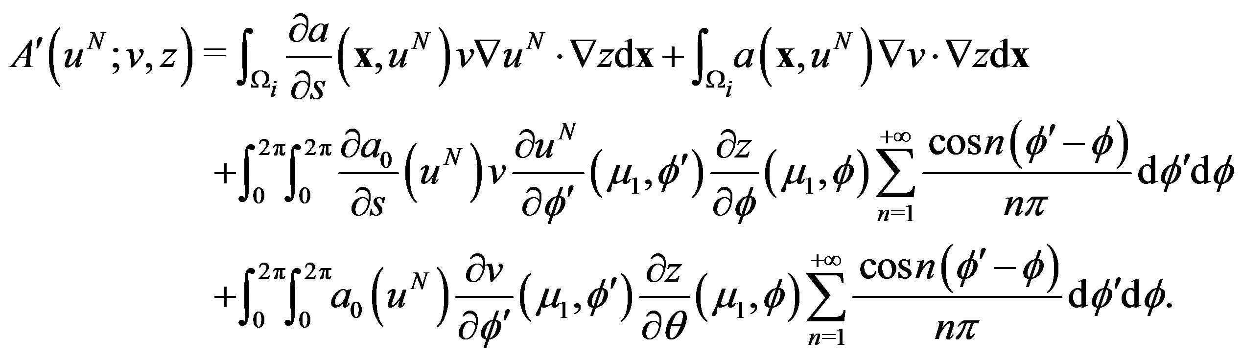
Now we introduce the bilinear form  and
and  defined by
Let  be the dual space of
 . By (1.2) and continuity of
 , we obtain that
  is bounded in
 . Then there exists an operator
  such that
 (3.21)
Similar with the proof of [10], we have the lemma as follows
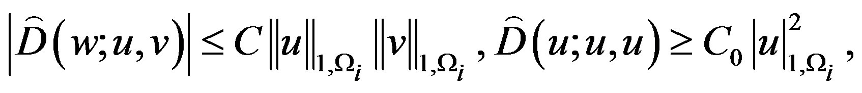
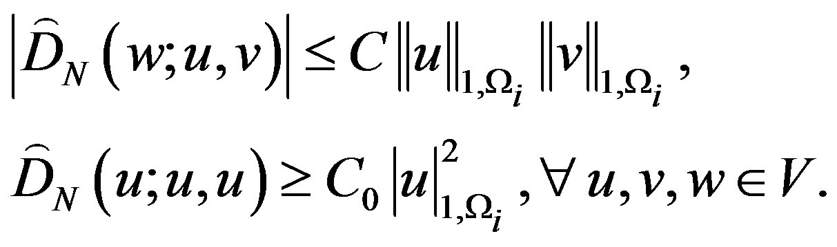
Lemma 3.5 The bilinear form  defined by
  satisfies the following inequality
 (3.22)
where  is a sufficient large constant and
 .
.
We assume that
 (3.23)
Let  be the canonical injection. Since
  is compactly embedded in
 , we have that the operator
  defined by
  is also compact. By (3.21) and (3.23) and
  satisfies the property of
 , we obtain that
  is an isomorphism.
By the conditions (3.2), (3.22), (3.23) and Theorem 10.1.2 of [20], one can get that there exists , such that the following inequality is satisfied
 (3.24)
for some constant  independent of
 .
.
We define the Galerkin projection with respect to ,
, 
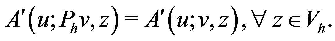
Then the operator satisfies
 (3.25)
We define the set
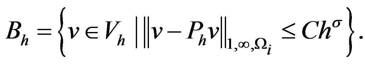
Lemma 3.6  is a solution of (3.14) if and only if the following equation
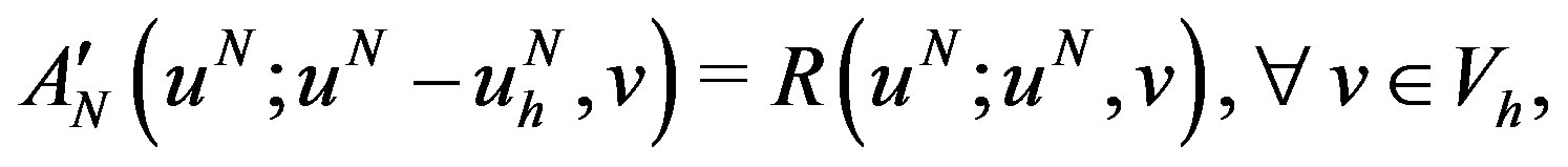
holds, where
with ,
, .
.
Proof. Let , then by
and

We can get the desired result.
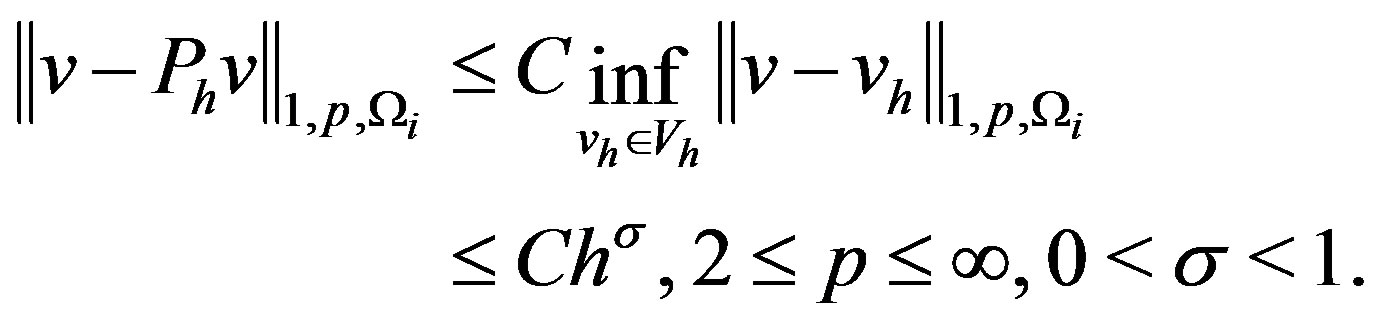
Let . Then following [10,11], we have
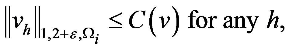
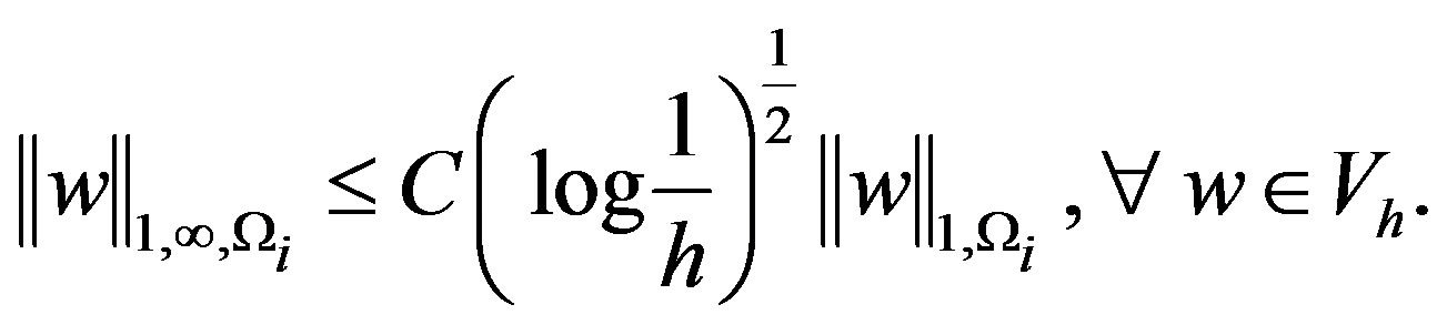
Lemma 3.7 There exists a positive constant C independent of h, such that
We also have the following result.
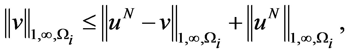
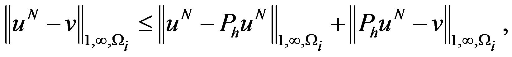
Lemma 3.8 
Proof For any , we only need to show that
 .
.
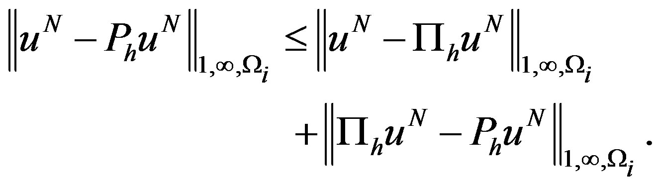
Since  is regular and quasi-uniform, referring to [19], we obtain the following inverse inequality
Combining the above inequalities with the definition of  and (3.26), we obtain
By the definition of , we get the desired result.
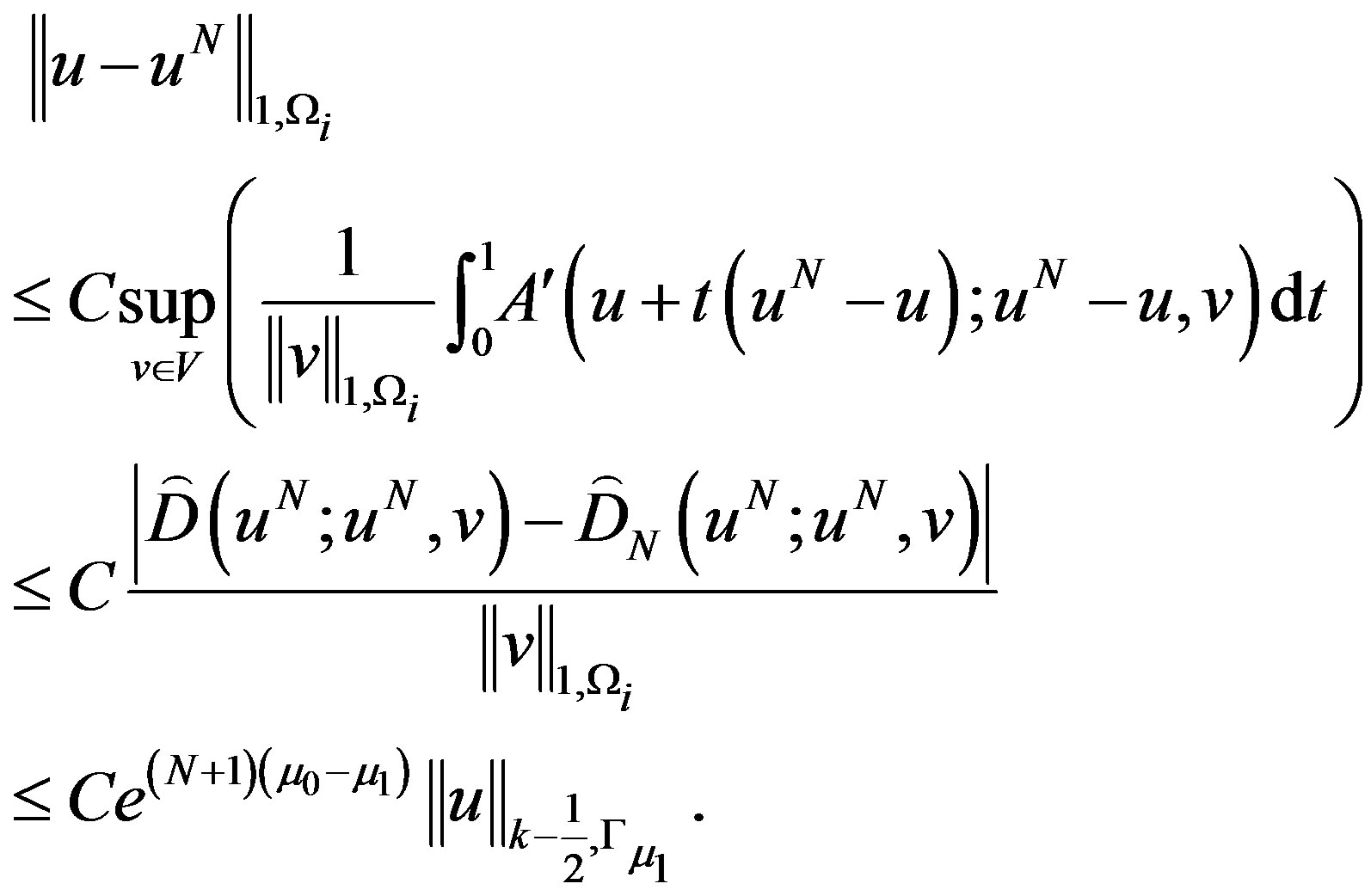
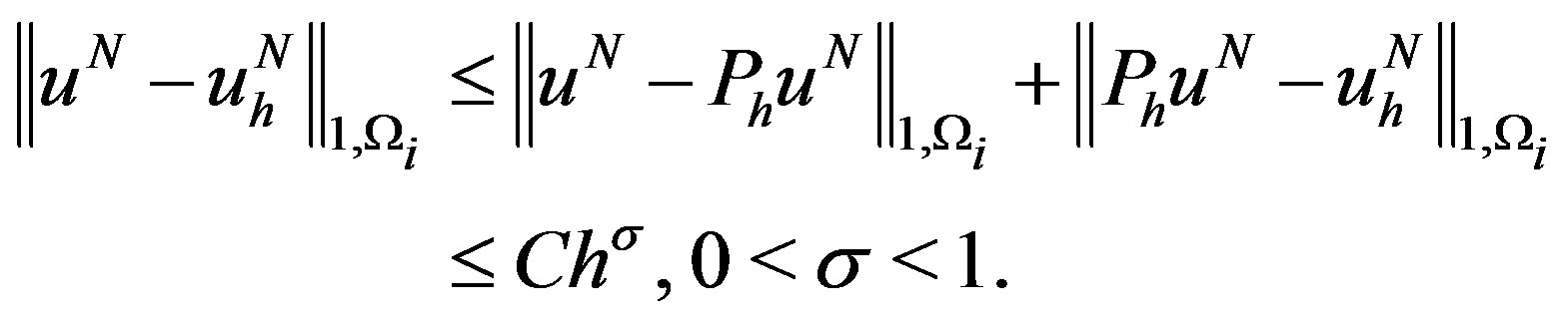
Theorem 3.2 Assume  be the solution of (1), with
 ,
,  , and we also assume that
 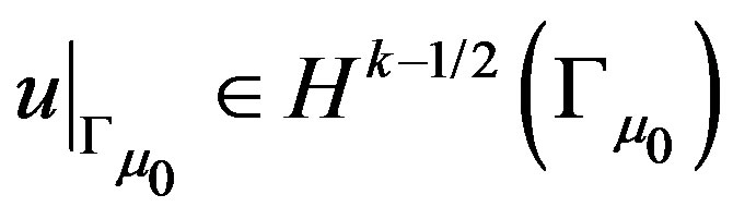 and
and satisfies (3.23). With sufficiently small
 , the finite element equation (3.16) has the approximate solution
  such that
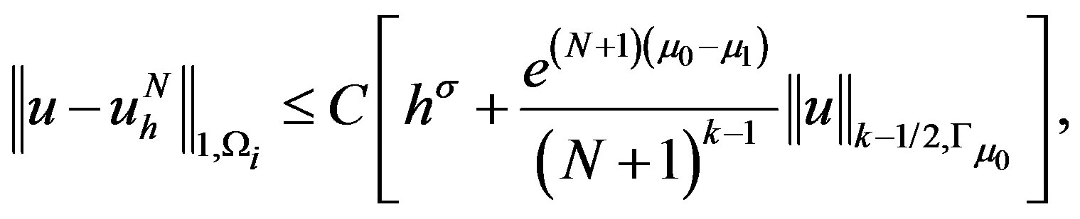
where C is a constant independent of h and N.
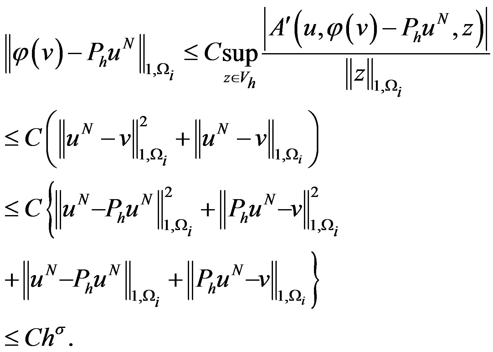
Proof Firstly, for any , we have
Then by (3.12), we have
Let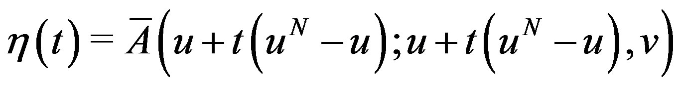 , we have
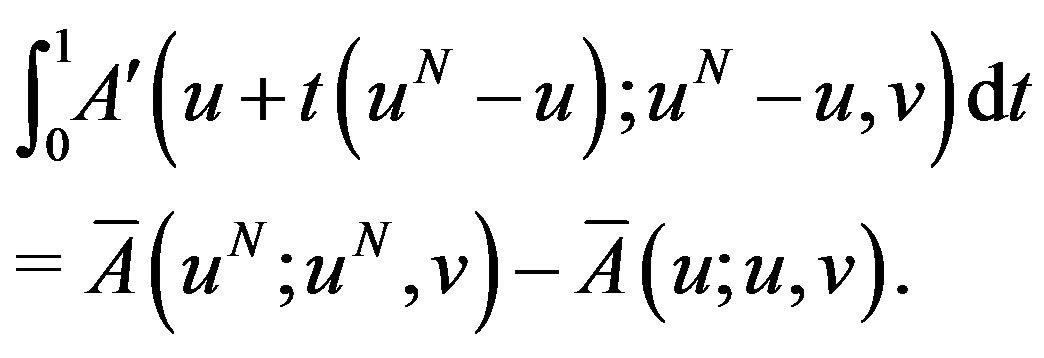
From (3.2), (3.22), (3.23) and [20], we obtain
 (3.26)
We denote a nonlinear mapping , which satisfies that for any given
 ,
,  is the unique solution of
 (3.27)
Therefore, we have
Combining the above equation with (3.25), we obtain the operator is continuous, i.e.,
Next, we assume that , then by Lemma 3.8, we have that
 . By the definition of
 , (3.27) can be rewritten as

Then, from (3.24), Lemma 3.6 and Lemma 3.7, we have
This implies that . And since
  is also continuous, following from Brouwer’s fixed theorem, one can obtain that there exists
 , such that
 . From
Lemma 3.6, we deduce that  is the solution of (3.16). What’s more, by (3.25) and the fact
 , we obtain
 (3.28)
Combining (3.26) with (3.28), one can obtain

This completes the proof.
4. Numerical Examples
In this section, we shall give some examples to confirm our theoretical results. In the following, we choose the finite element space as given in (3.16). For simplicity, we let
Example 4.1 We assume the exterior domain  with elliptical boundary
Now we consider the problem
 (4.1)
(4.1)
when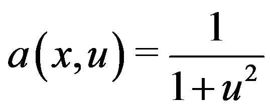 ,
,  and
and .
.
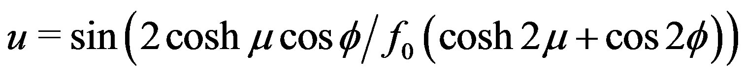
The exact solution of Example 4.1 is
 .
.
The numerical results are given in Figures 1 and 2 and Table 1.
Example 4.2 Similar with Example 4.1,  and
and  are replaced by
and  respectively.
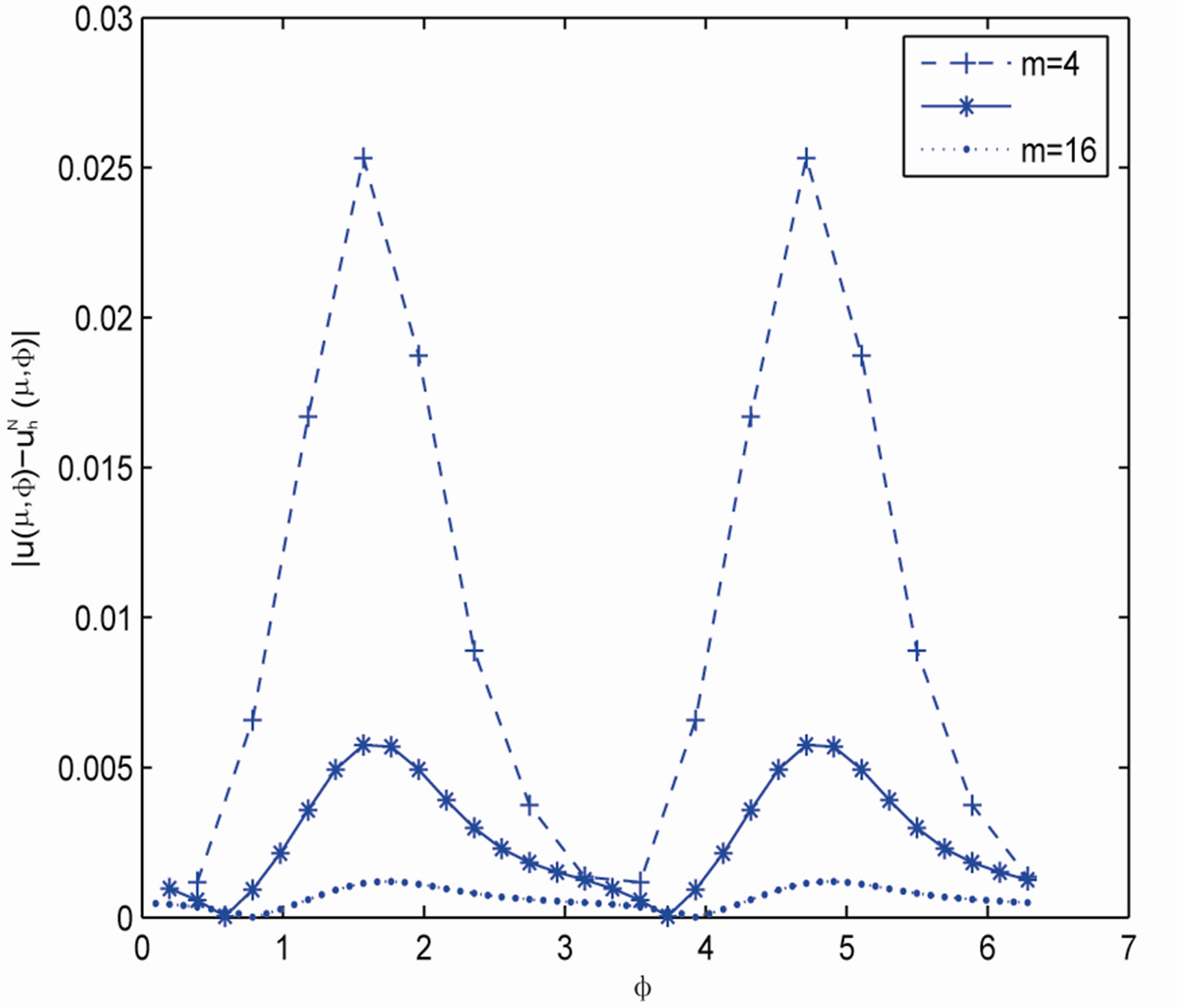
Figure 1. Example 4.1 with N = 16, µ1 = 1.7.
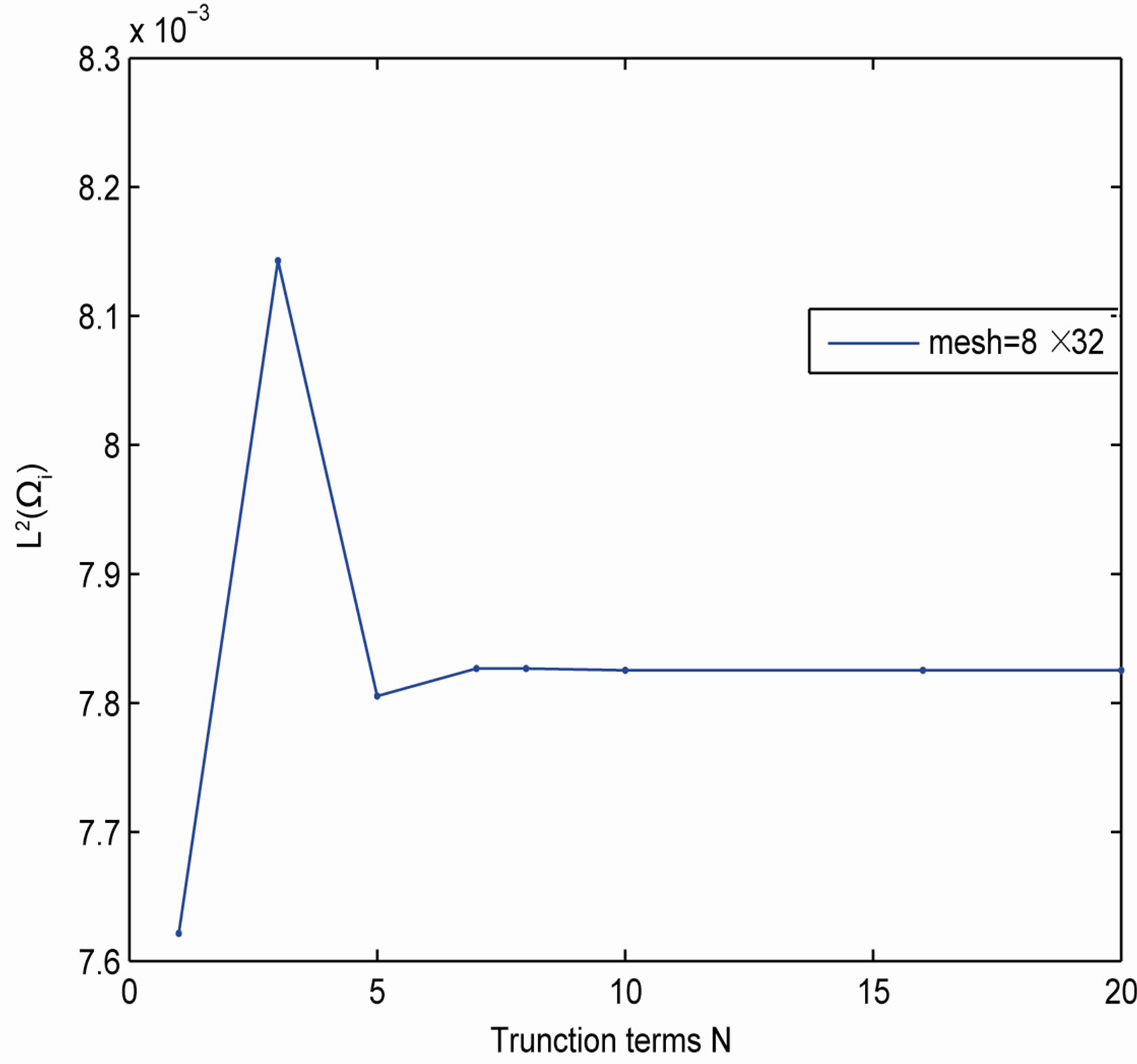
Figure 2. Example 4.1 with different N.
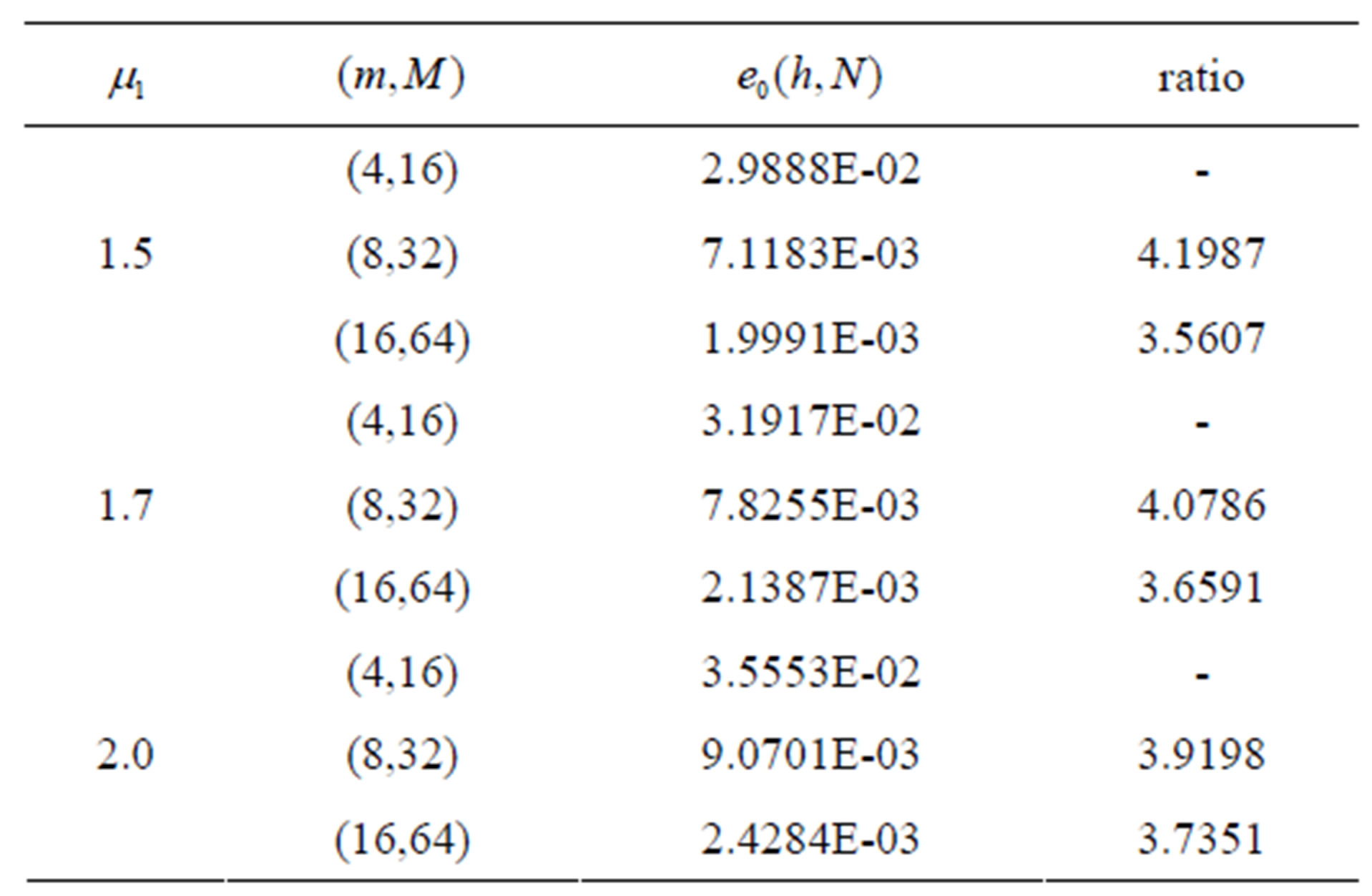
Table 1. The errors with N = 16 for Example 4.1.
The exact solution of Example 4.2 is
 .
.
The numerical results are given in Figure 3, Figure 4 and Table 2.
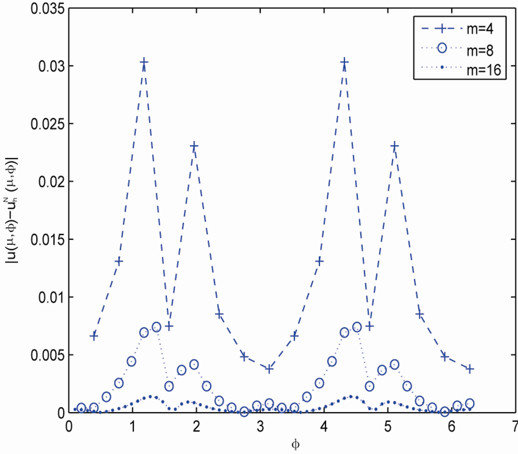
Figure 3. Example 4.2 with N = 6, µ1 = 1.0.
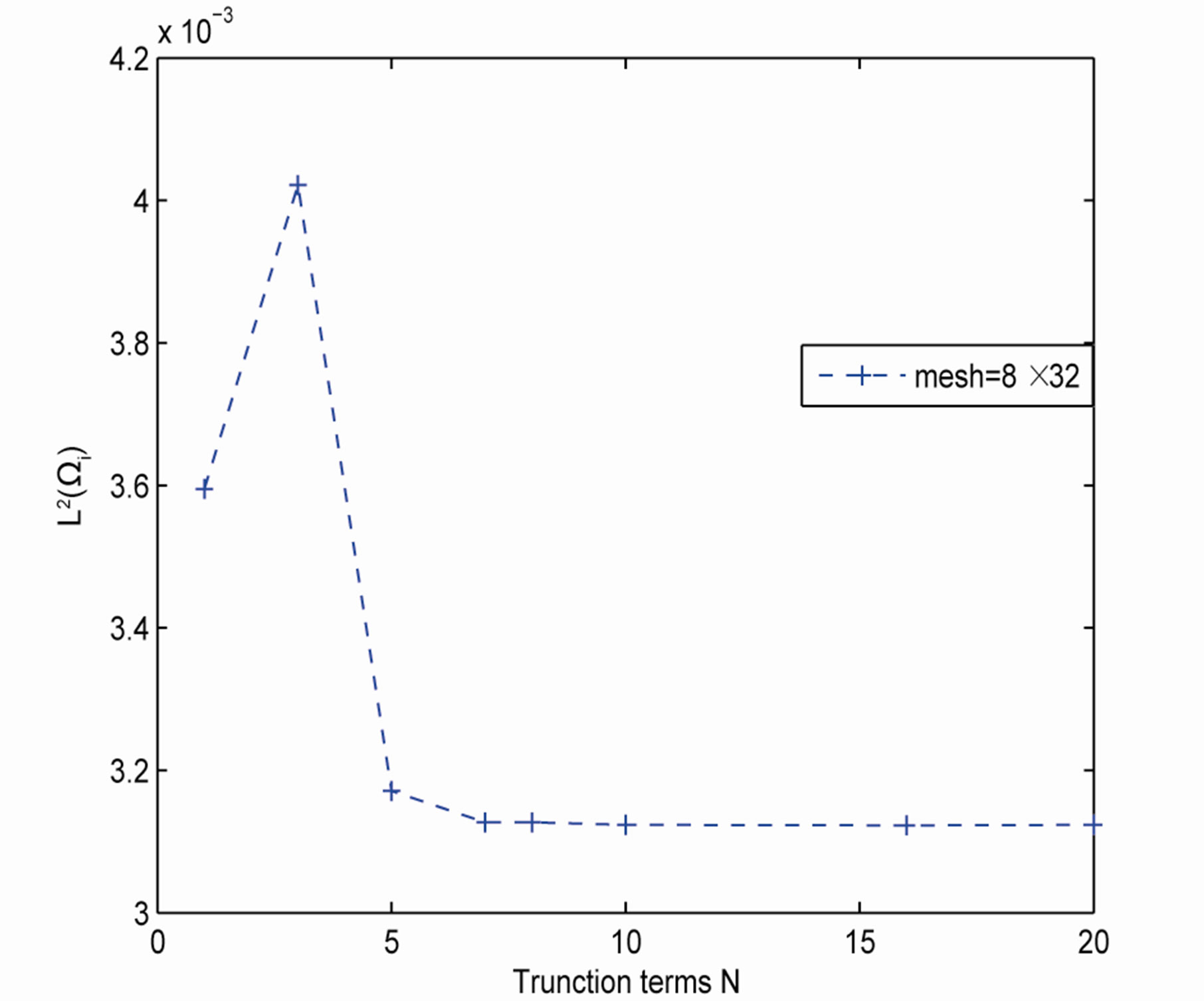
Figure 4. Example 4.2 with different N.
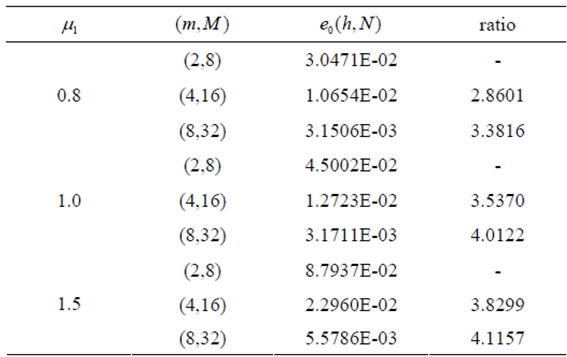
Table 2. The errors with N = 6 for Example 4.2.
Example 4.3 We assume the exterior domain  with elliptical boundary
Now we consider the problem
 (4.2)
(4.2)
when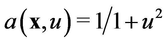 ,
,  and
and
The exact solution of Example 4.3 is
 .
.
The numerical results are given in Figures 5 and 6 and Table 3.
Example 4.4 Similar with Example 4.3,  and
and  are replaced by
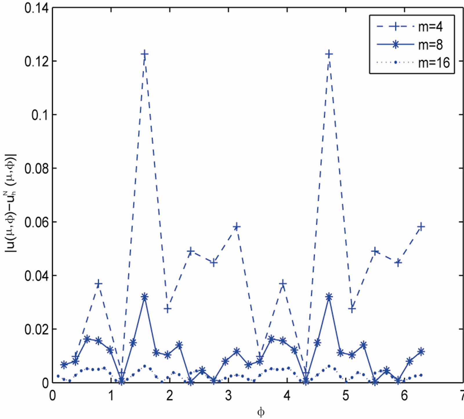
Figure 5. Example 4.3 with N = 10, ε = 0.005.
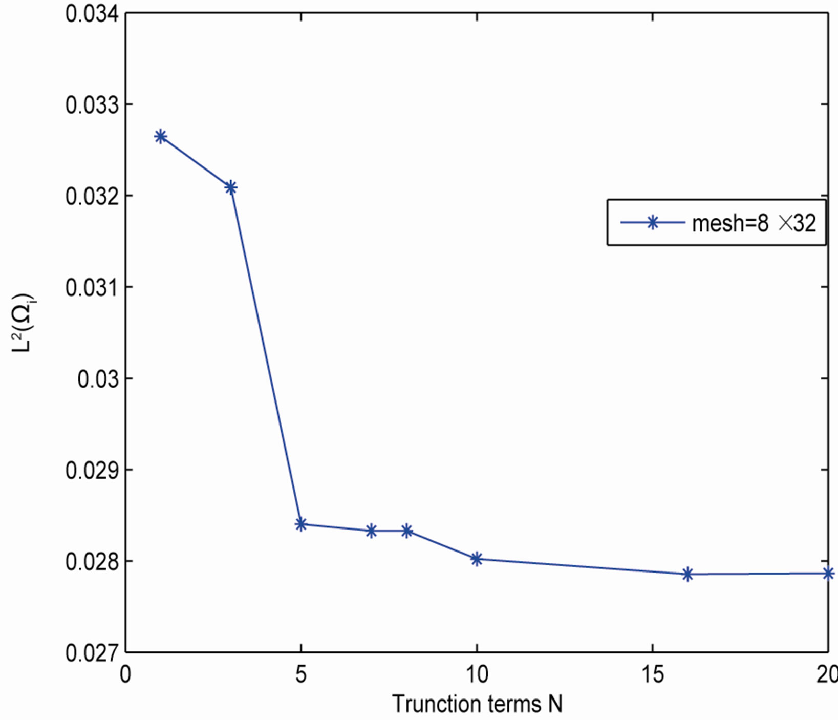
Figure 6. Example 4.3 with different N.

and  respectively. And we take
The exact solution of Example 4.3 is
 .
.
The numerical results are given in Figures 7 and 8 and Table 4.
From the numerical results, one obtains that the numerical errors can be affected by the order of artificial boundary condition, the mesh of the domain and the location of the artificial boundary, and it can be reduced by increasing the order of the artificial boundary condition and refining the mesh. What’s more, the convergence rate of anisotropic problems can also be affected by the choice of as it is shown in Tables 3 and 4. The numerical results are in agreement with the error analysis we obtain and show the efficiency of the coupling method.
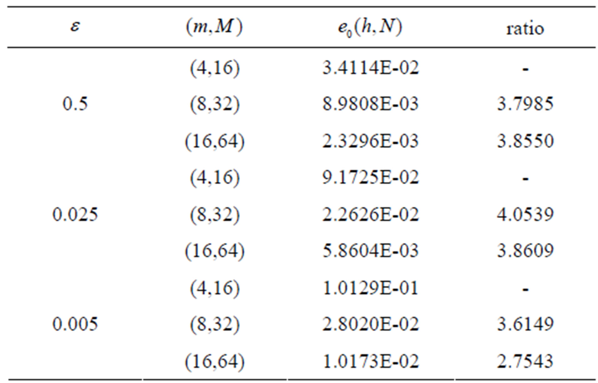
Table 3. The errors with N = 10 for Example 4.3.
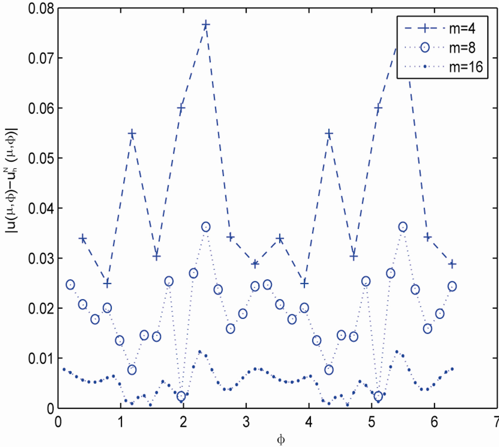
Figure 7. Example 4.4 with N = 5, ε = 0.05.
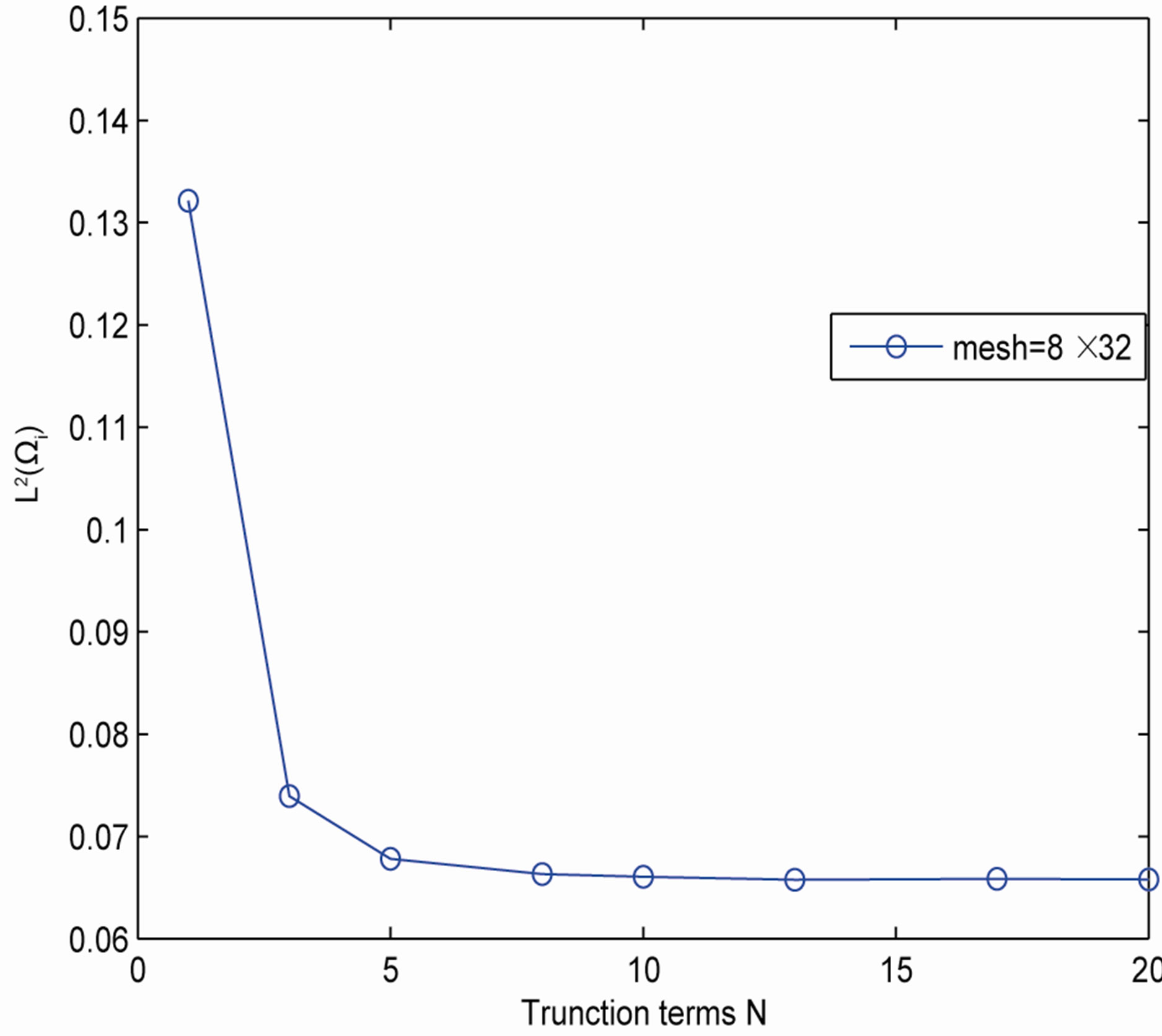
Figure 8. Example 4.4 with different N.
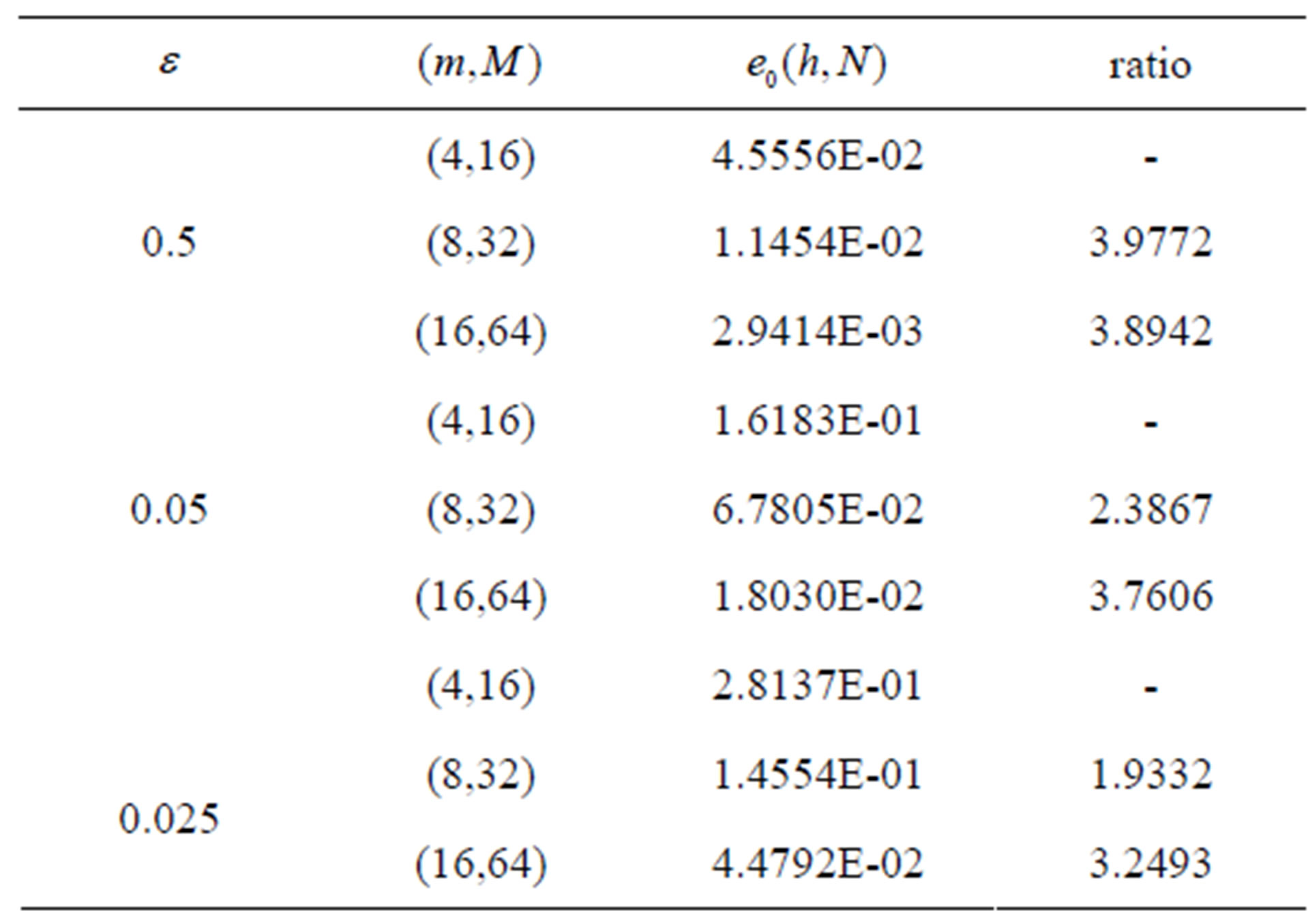
Table 4. The errors with N = 10 for Example 4.4.
5. Acknowledgements
This research was partly supported by the National Natural Science Foundation of China (contact/grant number: 10871100,11071109). The computations in this paper have been carried out in the Jiangsu Provincial Key Laboratory for Numerical Simulation of Large Scale Complex Systems. The authors express their thanks to them.
REFERENCES
- K. Feng, “Finite Element Method and Natural Boundary Reduction,” Proceedings of the International Congress of Mathematicians, Warsaw, 1983, pp. 1439-1453.
- D. H. Yu, “Natural Boundary Integral Method and its Applications,” Science Press & Kluwer Academic Publishers, Amsterdam, 2002.
- H. D. Han, Z. Y. Huang and D. S. Yin, “Exact Artificial Boundary Conditions for Quasilinear Elliptic Equations in Unbounded Domains,” Communications in Mathematical Science, Vol. 6, No. 1, 2008, pp. 71-83.
- H. D. Han and X. N. Wu, “The Artificial Boundary Method—Numerical Solutions of Partial Differential Equations on Unbounded Domains,” in Chinese, Tsinghua University Press, Beijing, 2010.
- M. J. Grote and J. B. Keller, “On Non-Reflecting Boundary Conditions,” Journal of Computational Physics, Vol. 122, No. 2, 1995, pp. 231-243. doi:10.1006/jcph.1995.1210
- M. J. Grote and J. B. Keller, “Exact non-Reflecting Boundary Conditions, Journal of Computational Physics, Vol. 82, No. 1, 1989, pp. 172-192. doi:10.1016/0021-9991(89)90041-7
- Q. K. Du and M. X. Tang, “Exact and Approximate Artificial Boundary Conditions for the Hyperbolic Problems in Unbounded Domains,” Applied Mathematics and Computation, Vol. 169, No. 1, 2005, pp. 544-562. doi:10.1016/j.amc.2004.09.074
- G. N. Gatica and G. C. Hsiao, “On the coupled BEM and FEM for a Nonlinear Exterior Dirichlet problem in R2,” Numerische Mathematik, Vol. 61, No. 1, 1992, pp. 171- 214. doi:10.1007/BF01385504
- Z. P. Wu, T. Kang and D. H. Yu, “On the coupled NBEM and FEM for a class of Nonlinear Exterior Dirichlet problem in R2,” Science in China Series A, Mathematics, Vol. 47, No. 1, 2004, pp. 181-189.
- D. J. Liu and D. H. Yu, “A FEM-BEM formulation for an Exterior Quasilinear Elliptic Problem in the plane,” Journal of Computational Mathematics, Vol. 26, No. 3, 2008, pp. 378-389.
- S. Meddahi, M. Gonzalez and P. Perez, “On a FEM-BEM formulation for an Exterior Quasilinear Problem in the plane,” SIAM Journal on Numerical Analysis, Vol. 37, No. 6, 2000, pp. 1820-1837. doi:10.1137/S0036142998335364
- I. Hlavacek and M. Krzek, “A note on the Neumann problem for a Quasilinear Elliptic Problem of a Nonmonotone Type,” Journal of Mathematical Analysis and Application, Vol. 211, No. 1, 1997, pp. 365-369. doi:10.1006/jmaa.1997.5447
- G. Ben-Porat and D. Givoli, “Solution of Unbounded Domain Problems Using Elliptic Artificial Boundaries,” Communications in Numerical Methods in Engineering, Vol. 11, No. 9, 1995, pp. 735-741. doi:10.1002/cnm.1640110904
- D. H. Yu and Z. P. Jia, “Natural Integral Operator on Elliptic Boundary and the Coupling Method for an Anisotropic Problem,” in Chinese, Mathematic Numerica Sinica, Vol. 24, No. 3, 2002, pp. 375-384.
- J. M. Wu and D. H. Yu, “The Natural Boundary Element Method for Exterior Elliptic Problem,” in Chinese, Mathematic Numerica Sinica, Vol. 22, 2000, pp. 355-368.
- D. B. Ingham and M. A. Kelmanson, “Boundary Integral Equation Analysis of Singular, Potential, and Biharmonic Problems, Lecture Notes in Engineer,” Springer Verlag, Berlin, 1984.
- G. N. Gatica and G. C. Hsiao, “Boundary-Field Equation Methods for a class of Nonlinear Problems, Pitman Research Notes in Mathematics Series 331,” Longman, Harlow, 1995.
- I. Hlavacek, M. Krlzek and J. Maly, “On Galerkin approximations of a Quasi-Linear Nonpotential Elliptic Problem of a Nonmonotone Type,” Journal of Mathematical Analysis and Application, Vol. 184, No. 1, 1994, pp. 168-189. doi:10.1006/jmaa.1994.1192
- J. Xu, “Theory of Multilevel Methods,” Ph.D. Thesis, Cornell University, Ithaca, 1989.
- C. Chen and J. Zhou, “Boundary Element Methods,” Academic Press, London, 1992.
NOTES
*This work is supported by the National Natural Science Foundation of China, contact/grant number 10871100 and 11071109; Foundation for Innovative Program of Jiangsu Province, contact/grant number CXZZ12_0383, CXZZ11_0870.