Achievable Rate Regions for Orthogonally Multiplexed MIMO Broadcast Channels with Multi-Dimensional Modulation

doi:10.4236/ijcns.2010.31001

Int. J. Communications, Network and System Sciences, 2010, 3, 1-18

doi:10.4236/ijcns.2010.31001 blished Online January 2010 (http://www.SciRP.org/journal/ijcns/).

1

Pu

Achievable Rate Regions for Orthogonally Multiplexed

MIMO Broadcast Channels with Multi-Dimensional

Modulation

Marthe KASSOUF, Harry LEIB

Department of Electrical and Computer Engineering, McGill University, Montreal, Canada

Email: marthe.kassouf@mail.mcgill.ca, harry.leib@mcgill.ca

Received July 23, 2009; revised September 12, 2009; accepted November 27, 2009

Abstract

In this work, we consider a multi-antenna channel with orthogonally multiplexed non-cooperative users, and

present its achievable information rate regions with and without channel knowledge at the transmitter. With

an informed transmitter, we maximize the rate for each user. With an uninformed transmitter, we consider

the optimal power allocation that causes the fastest convergence to zero of the fraction of channels whose

mutual information is less than any given rate as the transmitter channel knowledge converges to zero. We

assume a deterministic space and time dispersive multipath channel with multiple transmit and receive an-

tennas, generating an orthogonally multiplexed Multiple-Input Multiple-Output (MIMO) broadcast system.

Under limited transmit power; we consider different user specific space-time modulation formats that repre-

sent assignments of signal dimensions to transmit antennas. For the two-user orthogonally multiplexed

MIMO broadcast channels, the achievable rate regions, with and without transmitter channel knowledge,

evolve from a triangular region at low SNR to a rectangular region at high SNR. We also investigate the

maximum sum rate for these regions and derive the associated power allocations at low and high SNR. Fur-

thermore, we present numerical results for a two-user system that illustrate the effects of channel knowledge

at the transmitter, the multi-dimensional space-time modulation format and features of the multipath channel.

Keywords: MIMO Channels, Broadcast Systems, Capacity Region, Space-Time Coding

1. Introduction

Multiple-Input Multiple-Output (MIMO) systems, em-

ploying multiple antennas at the transmitter and receiver,

have been shown to yield significant capacity gains for

single-user channels [1]. A gain in the capacity of MIMO

channels is also observed when increasing the number of

multipath components [2–4]. Furthermore, channel know-

ledge at the transmitter has been shown to increase ca-

pacity more significantly at low SNR [5,6]. These fa-

vorable features trigerred a considerable interest in the

application of MIMO technology to multi-user systems

as well.

The capacity region of the two-user scalar orthogonal

broadcast channel (BC) is shown in [7] to be a rectangle

generated by the set of jointly achievable mutual infor-

mation rate pairs. A larger capacity region may be ob-

tained by allowing multi-user data superposition instead

of simple time sharing [8]. Assuming perfect channel

state information (CSI) at transmitter and receiver, the

optimality of Code Division Multiple Access (CDMA)

with successive decoding has been established in [9,10]

for flat and frequency selective fading channels. MIMO

broadcast channels (BCs) belong to the class of non-

degraded broadcast channels, thus, making the evalua-

tion of their capacity regions very difficult. Superposi-

tion coding does not apply to non-degraded broadcast

channels because users may employ different rates mak-

ing successive decoding quite difficult if not impossible

[11]. However, this reference shows that a capacity re-

gion for broadcast channels can be achieved by using a

coding technique, nicknamed dirty paper coding (DPC)

[12], where the interference is non -causally know n to the

transmitter and unknown to the receiver. The optimality

of DPC in terms of maximizing the sum rate was proved

in [13] for a constant two-user BC with single-antenna

receivers, and known channel at the transmitter as well

as all receivers. Generalizations of results from [13] to

M. KASSOUF ET AL.

2

systems with arbitrary number of users and multiple

transmit and receive antennas has been carried out inde-

pendently in [14] and [15]. The sum rate optimality of

DPC for Gaussian MIMO BCs has been investigated in

[16–18] using the duality [19] between the DPC rate re-

gion of the MIMO BC and the capacity region of a

Gaussian MIMO MAC with similar power constraint. In

[20] it was shown that the DPC rate region is in fact the

MIMO BC capacity region. Scaling laws of the sum rate

for block fading Rayleigh MIMO BCs with large number

of users are considered in [21] using DPC, Time Divi-

sion Multiple Access (TDMA) and beamforming. The

rate balancing problem (i.e. the selection of the capacity

region boundary point that satisfies given constraints on

the ratios between the users’ rates) is considered in [22],

which also provides optimal and suboptimal algorithms

for MIMO BCs employing Orthogonal Frequency Divi-

sion Multiplexing (OFDM) transmission.

In this work, we consider a MIMO BC with ortho-

gonally multiplexed non-cooperating users who employ

space-time modulation. As in [23,24], we assume a

non-fading space and time dispersive multipath envi-

ronment. These schemes model the downlink of cellular

communication systems with orthogonal user multiplex-

ing. We consider a deterministic channel model since it

provides an insight to the behaviour of the capacity re-

gion with respect to the numb er of anten na and multipath

components, and often serves as a first step towards the

study of fading channels. We investigate the achievable

rate region of such orthogonally multiplexed broadcast

schemes with multi-dimensional space-time modulation,

where a transmitter attempts simultaneously to transfer

information to several u sers without mutual interference.

When the channel is known at the transmitter, we con-

sider the optimal power allocation that maximizes the

rate for each user. We also consider the power allocation

for each user that causes the fastest convergence to zero

of the fraction of channels whose mutual information is

less than any given rate, as the transmitter channel

knowledge goes to zero. For both cases, we investigate

the maximum sum rate. Considering a two-user broad-

cast system, we investigate the asymptotic behaviour of

the achievable rate regions at low and high SNR, and

provide the optimum power allocations that correspond

to the maximum sum rate. Illustrative numerical results

are provided for users having different propagation

channels, using different multi-dimensional space-time

modulation schemes and employing different number of

antennas. This paper is structured as follows. Section 2

presents the system model. The capacity region with

known channel at the transmitter is investigated in Sec-

tion 3. The case of unknown channel at the transmitter is

considered in Section 4. Section 5 presents some illustra-

tive numerical results. The conclusions follow in Section 6.

2. MIMO Broadcast Multipath Channels

with Space-Time Modulation

In this paper, column vectors and matrices are repre-

sented by lower-case and upper-case bold letters. The

component of a vector is denoted by [] Fur-

thermore,

th

dad

a



denotes the determinant of A, ⊗ denotes

the matrix Kronecker product, anddenotes the matrix

product. We use the following superscripts: ∗ for com-

plex conjugate, T for matrix transpose, and for

Hermitian conjugate. The vec() operator denotes the

stack in a single column vector of matrix columns or a

set of column vectors. The direct sum of matrices



†

n

1

n

ii

{}





n

is denoted by ]

. The vertical stack of

matrices with equal number of columns

1[

n

ii

diag



1

n

ii





n

in a

single matrix is denoted by . The -square

identity matrix is denoted by . The -dimensional

vectors

1[

i

]

n

i

stack

n

Ιn

in



e for 1, ,2,in







are defined as



,1



,,



2,



,,

T

inii



i



n 









e, with the Kronecker sym-

bol defined by





,1ij





if , and ij(,ij) 0





otherwise. For a scalar , we have .

Unless otherwise specified, the function denotes

the base-2 logarithm, and the superscript () refers to

the user in the system.

a{}



lo

max(

()

0, )

aa

g

k

th

k

We consider orthogonally multiplexed users, each

with power

K





k

P satisfying the constraint





1

k

K

kP





T

D

and affected by independent interference. Let

denote the total number of signal dimensions, with user

occupying a sub-space of dimensionality

T

P

k





k

D,

where





1

k

D

KD

T



. Each user employs a different sig-

nal sub-space. This model corresponds to an orthogonally

multiplexed MIMO broadcast channel (BC) without user

cooperation. For user , the propagation medium consists of

time resolvable multipath clusters following the 3GPP

space and time dispersive channel model [25]. The signal

paths of same cluster have equal propagation delays and are

resolved in spac e only. For use r we define the transmitted

and received signal vectors

k

]

T

()k

t

L

()

T

N

k

s() ()

() [

kk

ts()

12

(),(), ,

k

tst

()

k

s

t and ()

()t

k



z ()

[(zt

1k),

()

2(), ()

()

, ()]

k

R

kk

N

T

z

tzt ,

respectively, with and

T

N





k

R

N denoting the number of

transmit and receive ante nnas.

The continuous time channel model is specified by



 



1

k

t

L

kkkk

ll

l

tt









zFs i

k

t (1)

M. KASSOUF ET AL.

3

Figure 1. System model for user k.

Figure 2. Examples of dimension allocation schemes for user

with transmit antennas and k4

T

N= 4

(k)

D

= dimensions:

a) ATA, b) OTA, c) POTA with TOGs. 2

(k)

G

N=

where





k

l



and





k

l

F denote the propagation delay and

the





k

R

T

NN channel propagation matrix associated

with cluster . The interference vector



,, })

k

t

ll L({1























,k

R

kk

N

i

12

, ,ti()[

kk

ti]

T

ti is complex valued

zero mean white Gaussian, with autocovariance matrix











()k

†

))][()((

R

kk

ii o

NN



IEt t



 where









denote s the Di rac ’s delta functi on.

Consider the system model from [26] illustrated in

Figure 1. Assume a modulation process for user that

partitions the transmit antennas into groups called

Transmit Orthogonal Groups (TOGs), each sharing a

given subset of its

k





k

D signal dimensions. Hence each

TOG employs a different signal sub-space. Let





k

G

N

denote the number of TOGs (





1k

G

NN

T

), and





k

i

n

denote the number o f transmit anten nas in the TOG,

assumed to be adjacent. We assume an equal number of

signal dimensions per TOG,

th

i

 



k

Gk

G

D

DN

 and define

. The -dimensional complex input

vector

 

k

TG

DND

k



k

G

D









k

jnx for transmit antenna and the corre-

sponding

j





k

D-dimensional signal space vector









k

jny

are given by





() ()(

kk

T

jj

nn



yx



)

k

j

, with





 

kk

j

T

tN

e



k

GG

D

Ι

k

j

 and













({

j

1,

kk

jj G

tt N })

k

indi-

cating the TOG to which antenna belongs. The





k

j











k

G

Dk

D matrix determines the signal dimen-

sions (indexed by





{1, ,}

k

dD 

j

) that can be used on

transmit antenna by making





[(

k

j

)]

d

n0



y if the

signal dimension is not used on antenna , or

th

dj









[( )][

k( )]

k

j

djd

nn



yx





{1, ,}D

 k

G

 for d otherwise.

The multi-dimensional space-time modulation format is

determined by the matrices





1

}

T





1

k

G

N



{

kN

j

. With

and





k

G

NNT

we have the space-time modulation

formats Aggregate Transmit Antenna (ATA) and Or-

thogonal Transmit Antenna (OTA), respectively. The

space-time coding system [27] and the Alamouti transmit

diversity scheme with two transmit antennas [28] are

examples of ATA. The orthogonal transmit diversity

technique of IS 2000 [29,30 ] is an example of OTA. The

M. KASSOUF ET AL.

4

more general case corresponds to Par-

tially Orthogonal Tr ansmit Antenna (POTA), that can be

viewed as a combination of ATA and OTA. Examples of

ATA, OTA and POTA are illustrated in Figures 2(a), 2(b)

and 2(c), respectively.



(

k

GT

NN )

The transmitted waveform through antenna j is given

by

 

()(( ))()

T

kkk

jnj

s

tn









y



12

,,,

k

T

kkkk

D

tt t





 



tnT

dt

where

denotes user



,

ks

real orthogonal basis functions and is the symbol

rate. We assume no inter-symbol interference and perfect

synchronization at every receive antenna. Assuming per-

fect multipath time resolvability for each user as well as

perfect orthogonality between users, we have

1Τ

 



 



 

,,, ,

kkk k

dld l

tnTt nT

kk ll ddnn

 

 





  

 









,, ,1,,k

t

kk llL ,







,1,,

k

dd D

and . Since different TOGs employ different sig-

nal subspaces, user system is equivalent to

,nn

,

ks





k

G

N

parallel MIMO systems each consisting of a TOG and

the receiver. The overall Maximum Likelihood detection

complexity for user is the sum of his TOGs com-

plexities, each being exponential in . By reducing

each

k



k

i

n





k

i

n the overall complexity decreases. It is mini-

mum, and linear in when

T

N





1

k

i

n which corre-

sponds to OTA. Thus, increasing lowers complex-

ity and increases parallelism.



k

G

N

Let









k

ml n



r and









k

ml n



v denote the





k

D

th

-dimen-

sional discrete time channel output and noise vectors o f the

time re solvabl e cluster received on the antenna.

th

l m

Hence, the vectors













1

} )

T

k

N

jj

nn 

xx

 

11

} )

kk

t

RL

l

({

k

vec and

denote the input and

output of the discrete time channel defined by



({ }

kk

N

ml m

nvecnrr

























kkkk

nrHxvn



ml n

n (2)

with noise vector .Using



 

11

({{}} )

kk

t

R

kk

NL

m l

n vec

vv









1[

T

k

N]

k

j

diag 





, we have

















1

} )

T

N

jj

n({

kk

vecn



yy













[]

kk

Tnx. Assuming perfect multipath resolv-

ability, the













kkk

tR

DLN



()k

D

 discrete time channel

matrix





k

H can be seen as the stack of









kk

ND

R



submatrices each associated with a time resolvable

cluster. T herefore, we have

()k

D





 



 

1

[([] ]

[([ ]

k

t

k

t

kk

LT

ll

kk

LT

ll

stack





HFI



k



)

)]

k

D

FI





T









or, equivalently,

 





k

kk k

D







HCI (3)

Figure 3. Space and time dispersive MIMO channel model for user .

k

M. KASSOUF ET AL. 5

]

k

F

with . Using the 3GPP spatial chan-

nel model [25] illustrated in Figure 3, let denote

the number of propagation paths in cluster , with path

characterized by the gain coeffi-

cient



1[

k

t

k

L

ll

stack 

C



(0,, 1)

k

l

S 



k

l

S

l

ss





;

k

ls

G, angle of departure (AOD)





;;s

k

Tl



and angle

of arrival (AOA)





;;

k

R

ls



k



k

.The total number of propagation

paths for user is . The spaces between

adjacent transmit and receive antennas are denoted by

and



1

k

tk

L

ll

S



T

d

R

d. We use the notations

 

;2

k

ls

C

k

R

d











;; )

k

sin(

R

ls





and



;

2sin(

k

T

Tl

d





;;

k

)

s



ls  with



de-

noting the signal wavelength. The space signature vec-

tors at the receiver and transmitter are given by

and

and from [25] we can write



;

k

ls

a

jN

e

 

;;

(1)

[1,, ,

kk

R

ls ls

jjN

ee









;

1]

k

TlsT







]

k

Tb



;

k

ls



;k

ls

j



[1, e

, ,





k

l



F

. Subsequently, we define the

propagation matrix describing the

propagation between the TOG and the receiver of

user , such that



 

1†

0;; ;

()

k

Skkk

slslsls

G

ab

 

kk k

tR i

n

k

l







LN



k

i

C

th

i



















12

kkk

 CCC[]

k

G

N

C. Let





k

i

r

denote the rank of





k

i

C and define .

We also use

 

kk

ii

rr

()

1

k

G

N

T







k

i

M and





k

i

Q to denote the





k

i

n-square

unitary and diagonal matrices associated with the eigen-

value decomposition

 









k

i

M

††

i

M()(

kk

ii

CC )

k

Q

k

i

.

Assuming a memoryless channel, we can drop the de-

pendencies on the time index for the remainder of

this paper. Moreover, we consider orthogonally multi-

plexed broadcast MIMO channels with two users (

n

K

= 2)

for simplicity. The results can be generalized to broad-

cast systems with an arbitrary number of users. In the

next section, we investigate the capacity region assuming

that the transmitter and both receivers have perfect

knowledge of the channel propagation matrices





21

{}

k

k

C and the multi-dimensional space-time modula-

tion formats .



21

{}

k

k



3. Capacity Region with Known Channel at

the Transmitter

Let denote the input covariance

matrix of user constrained by



†

[()

kkk

E

xx

k

]









()

k

Tr P

k

. For a

fixed





k

, the input/output average mutual informa-

tion for (2) is maximized by a Gaussian input distribution

and it is given by [1]

 

 

†

0

1

(,)log(|( )|)

kkk

tR

kkkk k

LN D

IN





xrIHH

(4)

From [1,31], Shannon capacity is obtained by maximiz-

ing









(,

kk

Ixr) over all positive semidefinite input co-

variance matrices





k



satisfying









()

kk

Tr P

.

From [32], we have that this capacity is obtained using a

water-filling power allocation [31], and it is given by



 

;

11

1{log()}/Hz

kk

Gi

Nn

kkk

il

k

il

G

Cb

N







 ps (5)

where















;1 ;2;0

k

i

kk k

ii in

 

 denote the (real and

n-negative) ordered eigenvalues of no









†

()

k

i

CC

k

i

, and

the constant





k



satisfies



k

N





11

{

kk





Gi

n

il





1}

;

()

k

il







 



0

kk

G

k

NP

ND

. The corresponding input signal





k

]

x is zero

mean Gaussian with a block diagonal covariance matrix



1[

k

G

kk

N

ii

diag 





 where the









kk

iG

nD -square input

covariance matrix of TOG is given by i











 



†

1

01 ;

()

([{ }])(

k

G

k

i

kk

GG

kk

ii

D

kk k

n

lil i

DD

Ndiag









)



MI

IMI

that, using [33], reduces to











 



†

1

01 ;

[( )

([{()}])]

k

i

k

G

kk

ii

kk k

n

lili

D

Ndiag











M

MI

(6)

All rate pairs









12

(,RR)

such that













11

(,)RIxr

1

and













22

(,)xr

2

RI are achievable, and the capacity

region is the closure of all such rate pairs









12

(, )RR .

We specify the power allocation between the two

users by



1

p

T

P



, which is the fraction of power

allocated to user one. The fraction of power allocated

to user two is





2

1p

T

P



 . Using (5) and the nota-

tion





()

k

p

C



for





,1,2

k

Ck, the boundary of the

capacity region is a parametric curve in p



defined

by

M. KASSOUF ET AL.

6



 







 





11

22

1

11

11 ;

1

2

22

11 ;

2

1log/H

1log/ H

Gi

p

Nn

il il

G

p

Nn

il il

G

C

bps z

N

C

bps z

N





























(7)

such that

 



111

1

11

11 ;1

0

{}

Gi GpT

Nn

il il

N

P

ND







 

 and

 

 



222

22

1

11 ;2

0

(1 )

{()}

Gi Gp

Nn

il il

NP

ND













 T

with

[0,1]

p



. Using a time-sharing argument as in [31],

we have that the capacity region is convex-



, and

also continuous since continuity is an underlying

property of convexity [34]. Moreover, as p



in-

creases in the interval [0, 1],





1

P increases and





2

P

decreases, leading to an increase in





1(

p)C



and

decrease in





2()

p

C



, respectively. Hence,





1(

p)C



is

monotonically increasing with

p



while





2()

p

C



is

monotonically decreasing with

p



. It follows that



2()

p

C



is a monotonically decreasing function of





1()

p

C



.

In order to assess the transmission performance of a

multi-user system using a comparison of capacity regions,

we introduce the following definition:

Definition 1: A capacity or rate region is said to be

larger (respectively, smaller) than another region if the

former contains (respectively, is contained in) the latter

for the same power .

T

P

For a fixed p



(or ), [32] shows that for a single

user system



k

P





()

k

p

C



is maximized by ATA, and for





2

k

G

N merging TOGs cannot decrease





()

k

p

C



. It

follows that, for = 1, 2 and for a given

kp



, maxi-

mum, intermediate and minimum values for





()

k

p

C



are respectively obtained when user employs ATA,

POTA and OTA, provided that the POTA system can be

obtained from OTA by merging TOGs. A straightfor-

ward application of this result to the boundary points of

the capacity region (7) of the orthogonally multiplexed

MIMO BC leads to the following theorem:

k

Theorem 1: With channel known at the transmitter, the

capacity region is largest, intermediate and smallest

when the users employ ATA, POTA and OTA, respec-

tively.

Considering a transmitter with transmit antennas,

ATA represents a transmission strategy where there are

no constraints on the assignment of a signal dimension to

the transmit antennas. As such, with ATA a signal di-

mension can be used on all the antennas. For POTA, a

signal dimension is constrained to be used only on a

subset of antenn as, while for OTA it is constrained to be

used only on one antenna. Thus, as

T

N





k

G

N increases the

assignment of a signal dimension to transmit antennas is

more constrained, yielding a decrease or no change in the

capacity.

We now investigate the sum capacity. Given , we

use

T

P

;

p

s



to denote the power allocation that maximizes

the sum capacity. Define the maximum sum capacity











12

0,1(( )( ))

p

sp

CCC





max



p

, and let









12

s

(,

s

CC)

denote the point of the capacity region boundary that

corresponds to ;

p

s



. We have









12

s



s

CC . Using

the convexity property and considering the two-dimen-

sional plane defined by the axes

C





1

R and





2

R, the

point









12

(, )

ss

CC corresponds to the intersection of the

boundary of the capacity region









12



((

 

12

),()

pp

CC)

with the affine function

s

RRC. Thus,









1

(,

ss

CC

2

), is the point at which the support line to









1

(( 2

),())

pp

CC



has a slope equal to −1, and is lo-

cated at the most right of the capacity region.

Let





()

k

bT

E denote the transmitted energy per bit

when operating at capacity limits. We have





()

k

bT

E







()

k

p

CD

k

P





k

. The SNR per bit referenced

at the transmitter satisfies

0

(/)

bT

EN



 

0

()(/ )

k

kk

p

bT

k

PCEN

ND



 (8)

Next, we consider the capacity region and sum capac-

ity at low and high SNR.

3.1. Capacity Region at Low SNR

For user at low SNR only the eigenmodes corre-

sponding to the maximum eigenvalue

k

() max

k









 

;11

{{}} k

k

iG

kN

n

ij ji





()k

are active. Let denote the num-

ber of elements of {{ that are equal to

()k

r





1

k

G

N

i



;1

} }

k

i

kn

ij j



. Thus, usin g ( 8) and (5) we h a ve

M. KASSOUF ET AL. 7













()

0

()

()log(1(/ ))

kk

k

Gp

kk

pb

k

G

NC

r

CE

r

N











k

T

N

.

Equivalently, we can write



 

()

0

()

2

() ()()

21

(/) ()

(ln2) ln2

()

2

kk

p

G

k

NC

r

k

bT kk

Gp

k

G

p

kk k

EN NC

r

NC

r





















(9)

showing that





()

k

p

C



is linear in





0

(/)

k

b

EN

T

with

slope



() ()

2

(ln2)

kk





2

k

G

r

N

. As





()

k

p

C



→ 0, we have







0

/

bT

ENk→()

ln2

k



 (which corresponds to −1.6 − 10

). Furthermore, (7) becomes

()

10

log() d

k



B



 



 



1

11

1

1111

00

2

22

2

222

00

log(1) ln2

11

log(1) ln2

p

GpT pT

G

p

GpTp

G

C

NP P

r

NrNDND

C

NP

r

Nr NDND









































2

T

P

(10)

Hence, we have



11

0

1

ln2 ()

p

Tp

ND

PC





 leading to a

triangular capacity region (in the positive quadrant of the

two-dimensional plane defined by the axes





1

R and





2

R) bounded by the line

  

 

 



212

21

12 2

0

ln2

T

P

D

RR

DN





 



D

(11)

As → 0, the segment (11) converges to the point

(0, 0). 0

/

T

PN

We investigate the sum capacity at low SNR by con-

sidering three possible cases depending on the channel

parameters:

1)

If

 

 

21

12

>1

D





, then the right most support line









12

s

RR C

 

intersects the capacity region boundary

at



2

12

(, )

ss

CC 

;0

ps

2

0

(0,)

ln2

T

P

ND



, which corresponds to



with total transmit power allocated to user two

and a sum capacity



2

0

ln2

T

s

P

CND



.

2) If

 

 

21

121

D







 then the right most support line









12

s

RR C





 

intersects the capacity region boundary

at



1

12

(, )

ss

CC 

;1

ps

1

0

( ,0)

ln2

T

P

ND



, which corresponds to





with total transmit power allocated to user one

and a sum capacity



1

0

ln2

T

s

P

CND



.

3) If

 

 

21

121

D







 then the support line with slope −1

lies on the boundary of the capacity region (11), thus,

maximizing the sum capacity for any power allocation

p



. Hence, ;ps



may take arbitrary value in [0, 1] and









12

(,

ss

CC)

could be any point of the segment (11). The

sum capacity is given by



21

00

ln2 ln2

TT

s

PP

C.

ND ND







3.2. Capacity Region at High SNR

At high SNR, all









kk

TG

rD eigenmodes are active and the

channel capacity from (5) becomes



1

()

k

pk

G

CN





 

11;

log( )

kk

Gi kk

Nr

il il





 with

 



0

kk

kG

kk

T

NP

rND







 



1

11;

1[(

kk

Gik

Nr

ilil

k

T

r







 )]

. We define



1

k

G

kN

i

A





and



1;

log( )

k

ik

r

lil









 



1

11;

k

Gi

kk

r

ilil



1k

N

k

T

dr









yielding,

 



 



0

( )log()

kk

k

kk

G

T

pkkkk

GG T

NP

r

A

Cd

NN rND



 .

Equivalently, we have

 



 

0

( )log(1)

k

kk

kk G

T

pkkk

GT

N

rP

CX

NrNDd



 k

(12)

where

 



log( )

k

kk

T

kk

GG

r

A

X

NN

 d

. (13)

Using (8), we can write

C

M. KASSOUF ET AL.

8



 



 



 



 



[][]

022

(/) () ()

kk

kkkk

pp

GG

kk

TT

NC ANCA

k

rr

k

bT kk kk

Gp G

kk

TT

d

EN NC NC

rr









p

(14)

As









0

(),(/ )

kk

p

b

CE



 T

N increases exponentially,

making





0

(/)dB

k

bT

EN linear in





()

k

p

C



with slope



10

10log 23

kk

G

k

TT

NN

rr

G

k

. Furthermore, we prove the

following theorem in the appendix

Theorem 2: As , the asymptotic capacity

region with known channel at the transmitter becomes rec-

tangular, defined by the points (0, 0),

0

/

T

PN



2

20

(0,log( ))

TT

G

rP

N



1

10

(log(),0)



TT

G

rP

N

N and 1

10

(log(),



TT

G

rP

N

2

20

log( ))

TT

G

rP

N

N.

Hence, regardless of the space-time modulation format

the capacity region of the orthogonally multiplexed

MIMO broadcast channel converges to a rectangle, simi-

lar to that of ortho gonal broadcast channels [7]. Next we

investigate the sum capacity at high SNR for the follow-

ing cases:

1) 0< <1

p



: Using (12), we can write



2

1

()

p

dC







2

()

p

1

()

p

dC

d

dC





, which yields



  



 



1

11

201

12

22

02

()

() (1 )

G

pT

pG

p

T

N

dND P

dC r

dC N

dND P

r











. (15)

The denominator of (15) becomes zero for

 



22 2

0

2

1T

p

GT

rd ND

NP



 which is strictly larger

than 1, thus, making









12

((),()

p

CC



  



12

22 111

0

12

()}{

GG

TTT

NN

dD dD

Prr



}

N

, and as

0

/

T

PN



22

11

1

;2121

[1 ]

GG

T

ps

TGTG

NN

rr

rN rN







T

. (16)

Furthermore, from Theorem 2 we have that the capacity

region boundary points corresponding to





0, 1

p



con-

verge toward the upper right corner of the limiting rec-

tangle. Therefore, we have

 



1

12

10

(,)(log( ),

TT

ss

G

rP

CC N

N





2

20

log( ))

TT

G

rP

N

Nand

0

log( /)

s

T

C

P

N



12

(

TT

GG

rr

NN

)

. It is seen that both

s

Cand ;

p

s



depend

on the users space-time modulation formats as well as

the ranks of the TOGs propagation matrices without be-

ing dependent on the channel eigen values





;

k

il



.

2) 0

p





: From (15) the right derivative is such that



  



22

11221

00 0

12

()

[] [

()

p

pG

T

pT

dC N

dND dNDP

dC r



]







The support line at









12

((0), (0))CC is not unique and

has a slope that varies in the interval



2

0

1

()

[[], ]

()

p

dC









.

The lower bound of this interval is larger than −1 for

sufficiently large and hence, no support line at

the point

0

/

T

PN









1

((0),CC

2

(0)) can have a slope equal to −1.

It follows that









12

((0), (0))CC (for which 0

p





)

cannot be an intersection of the capacity region boundary

with the affine function









12

s

RRC, yielding

;0

ps





.

3) 1

p





: From (15) the left derivative is such that

)

p

differentiable

for all . It follows that the support line at

every point of the capacity region boundary with



0,1

p





10,

p







is unique and equal to the tangential line [34].

As , we have from (15) that

0

/

T

PN



2()

()

1

11

p

G



  



 

21

112 2

1

10 0

11

()

[]()[

()

p

pG

T

pT

dC N

dNDP dND

dC r



]



 

The support line at









12

((1), (1)CC



)is not unique and it

has a slope in

2

1

()

(,[]][0,)

()

p

dC











0

/

T

PN

 

12

((1), (1))CC

 that does

not include −1 if is sufficiently large. Hence,

no support line at the point can have a

slope equal to −1. It follows that









1

((1),CC

2

(1)

2

(1 )

p

T

p

pT

N

rG

r

N



dC







.The power allocation

that maximizes the sum capacity can be obtained by

solving ;

2

1

()

[]

()

pps

p

dC







1

, yielding



2

;2

{G

ps

T

N

r



 ) (for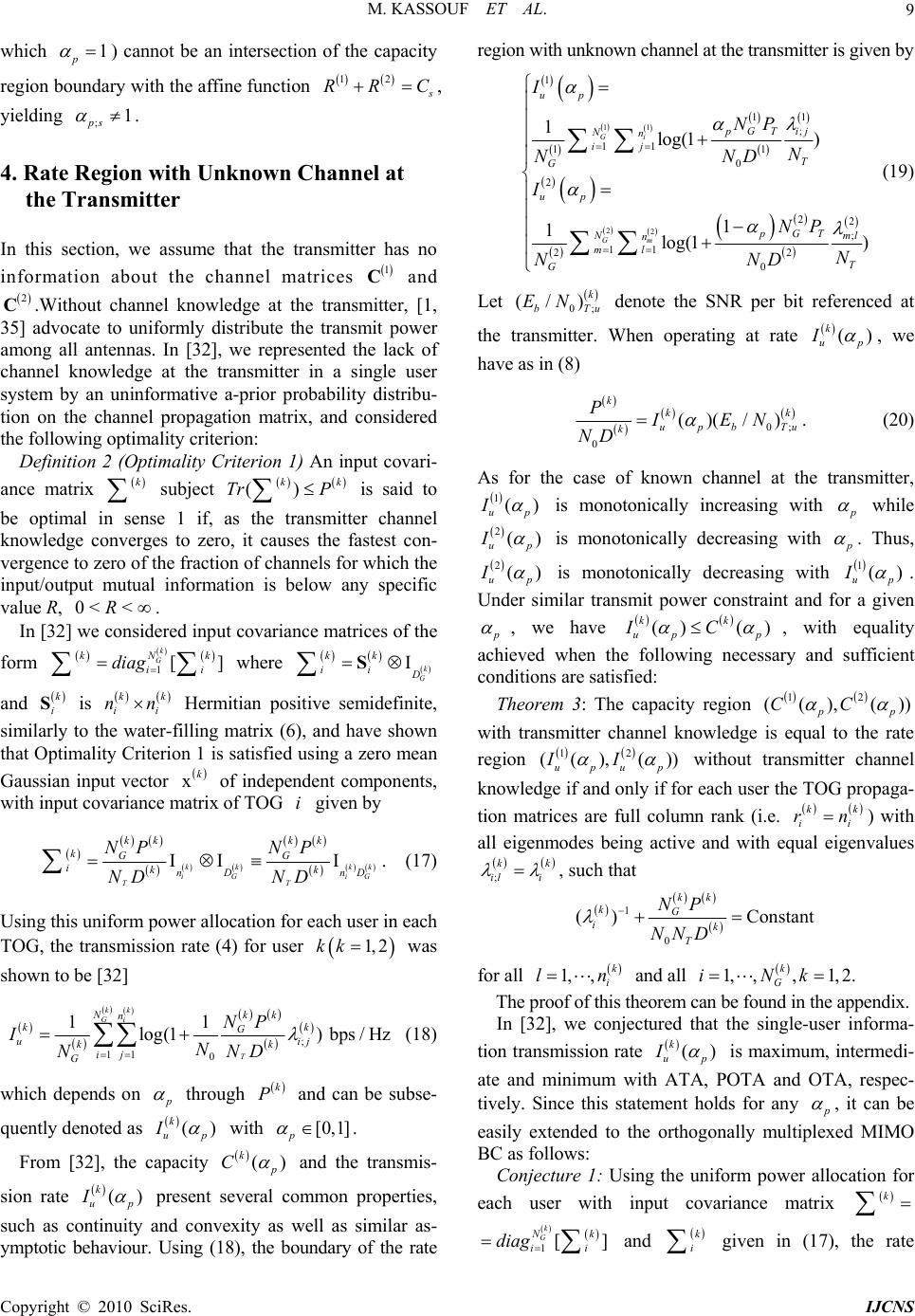

M. KASSOUF ET AL. 9

which 1

p



) cannot be an intersection of the capacity

region boundary with the affine function









12

s

RR C,

yielding ;ps 1



.

4. Rate Region with Unknown Channel at

the Transmitter

In this section, we assume that the transmitter has no

information about the channel matrices





1

C and





2

C.Without channel knowledge at the transmitter, [1,

35] advocate to uniformly distribute the transmit power

among all antennas. In [32], we represented the lack of

channel knowledge at the transmitter in a single user

system by an uninformative a-prior probability distribu-

tion on the channel propagation matrix, and considered

the following optimality criterion:

Definition 2 (Optimality Criterion 1) An input covari-

ance matrix





k

 subject









()

k



k

PTr is said to

be optimal in sense 1 if, as the transmitter channel

knowledge converges to zero, it causes the fastest con-

vergence to zero of the fraction of channels for which the

input/output mutual information is below any specific

value R, .

0<R





<

dia



In [32] we considered input covariance matrices of the

form where



1[

k

G

kk

N

ii

g



]











Ik

G

kk

ii

D

S



and





k

i

S



k

i

n

is Hermitian positive semidefinite,

similarly to the water-filling matrix (6), and have shown

that Optimality Criterion 1 is satisfied using a zero mean

Gaussian input vector



k

i

n





xk of independent components,

with input covariance matrix of TOG given by i

  



 



 

I

kk

ii

GG

kk

II

kk

TT

kk

GG

kk

nD nD

NP

ND





k

i





NP

ND . (17)

Using this uniform power allocation for each user in each

TOG, the transmission rate (4) for user was

shown to be [32]



1, 2kk



 



;

11

kk

Gi

Nn

ij

G

 0

11

log(1)bps/ Hz

T

kk

G

uij

kk

NP

IN

NND



 (18)

which depends on

p



through





k

P and can be subse-

quently denoted as





()

p

k

u

I



with [0,1]

p



.

From [32], the capacity





()

k

p

C



and the transmis-

sion rate





(

k

u

I)

p



present several common properties,

such as continuity and convexity as well as similar as-

ymptotic behaviour. Using (18), the boundary of the rate

region with unknown channel at the transm itter is given by









 



 



11

22

1

11

;

11

0

2

22

;

11

22

0

1log(1 )

1

1log(1 )

Gi

Gm

up

pGT ij

Nn

ij

T

G

up

pGT

mlNn

ml

T

G

I

NP

N

NND

I

NP

N

NND

































(19)

Let





0;

(/)

k

bT

EN u

denote the SNR per bit referenced at

the transmitter. When operating at rate





()

k

up

I



, we

have as in (8)



 

0;

0

()(/ )

k

upb T

k

PIEN

ND



k

u

. (20)

As for the case of known channel at the transmitter,





1()

up

I



is monotonically increasing with

p



while





2()

up

I



is monotonically decreasing with

p



. Thus,





2()

up

I



is monotonically decreasing with





1

I()

up



.

Under similar transmit power constraint and for a given

p



, we have









() ()

kk

up p

IC



, with equality

achieved when the following necessary and sufficient

conditions are satisfied:

Theorem 3: The capacity region









12

((), ()

pp

CC



)

with transmitter channel knowledge is equal to the rate

region









12

((),())

upu p

II



without transmitter channel

knowledge if and only if for each user the TOG propaga-

tion matrices are full column rank (i.e.









kk

rn

ii

) with

all eigenmodes being active and with equal eigenvalues









;

k

il

k

i



, such that

  



1

0

() Constan

kk

kG

ik

T

NP

NND



t

for all





1,,k

ln i and all





1,,,1, 2.

kk 

G

The proof of this theorem can be found in the appendix.

iN

In [32], we conjectured that the single-user informa-

tion transmission rate





()

k

up

I



is maximum, intermedi-

ate and minimum with ATA, POTA and OTA, respec-

tively. Since this statement holds for any

p



, it can be

easily extended to the orthogonally multiplexed MIMO

BC as follows:

Conjecture 1: Using the uniform power allocation for

each user with input covariance matrix





k







1[

k

Gk

N

ii

diag 

]



and





k

i



given in (17), the rate

C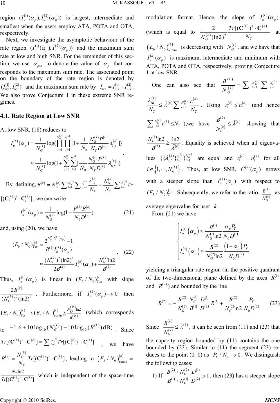

M. KASSOUF ET AL.

10

region









12

((),())

upu p

II



is largest, intermediate and

smallest when the users employ ATA, POTA and OTA,

respectively.

Next, we investigate the asymptotic behaviour of the

rate region









1

((),

upu

II



;ps

2

())

p



and the maximum sum

rate at low and high SNR. For the remainder of this sec-

tion, we use



 to denote the value of p



that cor-

re spo nds to th e max imu m su m rate. The associated point

on the boundary of the rate region is denoted by

and th e maximum sum rat e by



12

;;

(,

us u

II



)

s









12

;;us us

III

;us .

We also prove Conjecture 1 in these extreme SNR re-

gimes.

4.1. Rate Region at Low SNR

At low SNR, (18) reduces to



 



 



;

11 0

;

11 0

11

( )log([1])

11

log(1 [])

kk

Gi

kk

Gi

kk

Nn

kk

G

up ij

kk

ij

GT

kk

Nn

k

G

ij

kk

ij

GT

NP

IN

NN

NP

N

NND















D

.

By defining,

 



;

11 1

kk

k

Gi G

kk

ij

kk

NN

nG

Gi ji

TT

N

BN T

NN



 



r









†

[( )]

kk

ii

CC, we can write



 



0

1

() log(1)

kk

k

up k

G

PB

INND





k

(21)

and, using (20), we have











 



0;

22

21

(/) ()

() (ln2)ln2

()

2

kk

up

G

NI

k

bTukk

up

kk

k

GG

up

k

EN BI

NN

I

B









k

B

. (22)

Thus,





()

k

up

I



is linear in





0;

(/)

k

bT

EN u

with slope



22

(ln2)

k

B2

()

k

NG

. Furthermore, if





()

k

up

I



0 then









00

;min

ln2

//

k

u

k

NG

k

B

ENEN 

;

k

bb

Tu 

.6 10log



()]

kk

CC



(which corresponds

to . Since

, we have



10 1

1() 10log

G

N



†

1

[ [()

k

Gk

N

ii

Tr





CC



0()dB)

kk

B



†

]

k

i

Tr

 

†

[( )]

k

kkk

G

T

N

BTr

N

CC

, leading to







;min

k

0

/

bu

EN



 

†

ln2

[( )]

T

kk

N

CCTr which is independent of the space-time

modulation format. Hence, the slope of





()

k

up

I



(which is equal to



 

†

2

2[(

(ln2)

k

T

G

Tr

N

C)]

kk

C

at







0;min

/k

bu

EN is decreasing with





k

G

N, and we have that





()

k

up

I



is maximum, intermediate and minimum with

ATA, POTA and OTA, respectiv ely, proving Conjecture

1 at low SNR.

One can also see that



 

11

kk

Gi

k

G

B

N

Nn

il







 



;

k

il



1

k

G

k

kNi

i

TT

r

NN



. Using









k

i

rk

i

n (and hence



1

k

Gk

N

ii

r

T

N



),we have



k

G

B

N



k



 showing that



 

ln2 ln2

k

G

k

N

Bk



. Equality is achieved when all eigenva-

lues



;1

{{} k

kn

il l





1

}k

iG

N

i



 are equal and







i

n

k

i

rk

for all







1, ,k

G

iN. Thus, at low SNR,





()

k

p

C



grows

with a steeper slope than





()

up

k

I



with respect to





0

(/)

k

bT

EN . Subsequently, we refer to the ratio



k

G

B

N

as

average eigenvalue for user .

k

From (21) we have



 



1

2

22

ln2

up

G

11

0

1

pT

p

T

up

G

B

INN

P

B

ID















P

D

NN





yielding a triangular rate region (in the positive quadrant

of the two-dimensional plane defined by the axes





1

R

and





2

R) and bounded by the line

 



 

1

212

21

21 22

0

2

GT

NP

BD B

R

NBD ND

 2

ln

GG

R

N (23)

Since



k

G

B

N



, it can be seen from (11) and (23) that

the capacity region bounded by (11) contains the one

bounded by (23). Similar to (11) the segment (23) re-

duces to the point (0, 0) as . We distinguish

the following cases: 0

/

T

PN 0

1) If

 



22

1

112

/1

/

G

BN

D

BND

>, then (23) has a steeper slope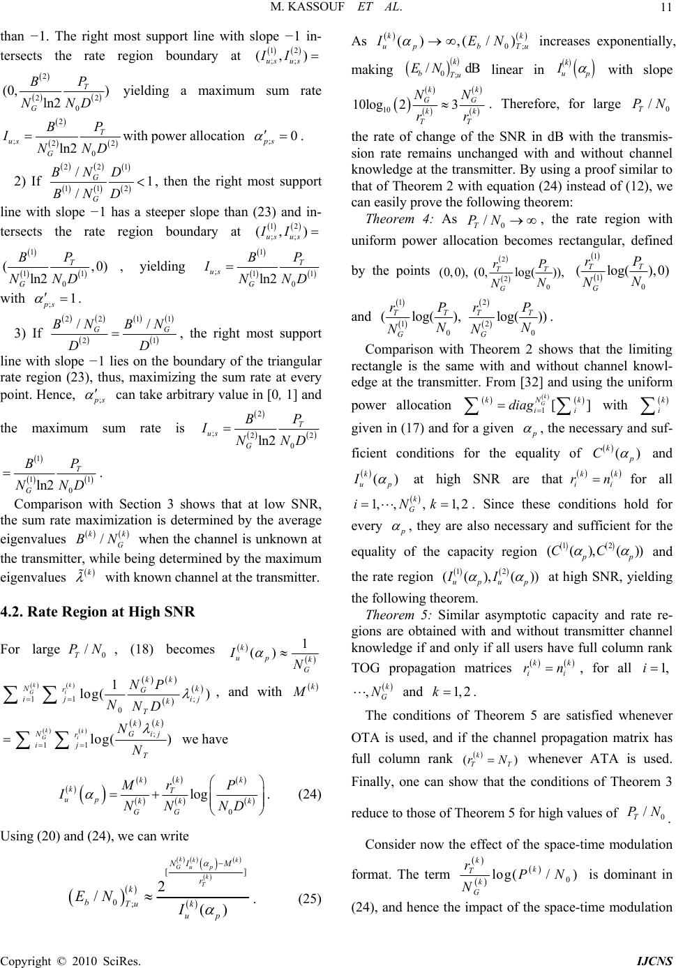

M. KASSOUF ET AL. 11

than −1. The right most support line with slope −1 in-

tersects the rate region boundary at









12

;;

(,)

us us

II





 

2

0

(0, )

ln2

T

G

P

B

NND

2

yielding a maximum sum rate



 

2

;2

0

ln2

T

us

G

P

B

INND

2

with power allocation ;0

ps







.

2) If

 



22

1

112

/1

/

G

BN

D

BND

<, then the right most support

line with slope −1 has a steeper slope than (23) and in-

tersects the rate region boundary at









12

;;

(,)

us us

II





 

1

11

0

(

ln2

T

G

P

B

NND

,0)

, yielding



 

1

11

0

ln2

T

G

P

B

NND

;us

I

with ;1

ps







.

3) If



 



22 1

2

//

G

BN BN

DD



1

G

, the right most support

line with slope −1 lies on the boundary of the triangular

rate region (23), thus, maximizing the sum rate at every

point. Hence, ;ps



 can take arbitrary value in [0, 1] and

the maximum sum rate is





 

2

0

ln2

T

G

P

B

NN

;22

us

ID







 

1

ln2

T

P

B

NND

11

0G

Comparison with Section 3 shows that at low SNR,

the sum rate maximization is determined by the average

eigenvalues

.









/

k

G

BN

k

when the channel is unknown at

the transmitter, while being determined by the maximum

eigenvalues





k



 with known channel at the transmitter.

4.2. Rate Region at High SNR

For large, (18) becomes

0

/

T

PN



1

()

up

N





k

G

I

 











11

lo g(

k

Gi

r

ij N

 ;

0

1)

kkk

k

NG

ij

k

NP

ND





T

, and with





k

M



 



;

11

lo g(

k

Gi

r

ij

 )

k

kk

Gij

N

T

N



 we have



0

log

k

kk

kT

up kk

GG

r

M

INN N



 



k

P

D







. (24)

Using (20) and (24), we can write







[]

0;

2

/()

kkk

up

G

k

T

NIM

r

k

bTu k

up

EN I





. (25)

As





0;

(),(/)

k

upb T

IE







k

u

N

increases exponentially,

making





0;

/dB

k

bTu

EN linear in







k

up

I



with slope



10

10log23

kk

G

k

TT

NN

rr

G

k

by

. Therefore, for large

the rate of change of the SNR in dB with the transmis-

sion rate remains unchanged with and without channel

knowledge at the transmitter. By using a proof similar to

that of Theorem 2 with equation (24) instead of (12), we

can easily prove the following theorem:

0

/

T

PN

Theorem 4: As , the rate region with

uniform power allocation becomes rectangular, defined

the points

0

/

T

PN



2

20

(0,0), (0,log()),

TT

G

rP

N



1

10

(log( ),0)

TT

G

rP

N

and



12

00

(log(), log())

TTT T

GG

rPrP

NN

.

Comparison with Theorem 2 shows that the limiting

rectangle is the same with and without channel knowl-

edge at the transmitter. From [32] and using the uniform

power allocation



1[

k

G

kk

N

ii

diag 

]



 with





k

i



given in (17) and for a given

p



, the necessary and suf-

ficient conditions for the equality of





(

k)

p

C



and





()

k

up

I



at high SNR are that









kk

i

n

i

rfor all





, 1,

k

Gk1, ,iN2. Since these conditions hold for

every

p



, they are also necessary and sufficient for the

equality of the capacity region and

the rate region



1

((CC

 

2

), (

p



))

p











12

((), ())

upu p

II



at high SNR, yielding

the following theorem.

Theorem 5: Similar asymptotic capacity and rate re-

gions are obtained with and without transmitter channel

knowledge if and only if all users have full column rank

TOG propagation matrices , for all

 

k

ii

rnk1,i







,k

G

N and 1, 2k



.

The conditions of Theorem 5 are satisfied whenever

OTA is used, and if the channel propagation matrix has

full column rank





(

k

T

rN)

T

whenever ATA is used.

Finally, one can show that the conditions of Theorem 3

reduce to those of Theorem 5 for high values of .

0

/

T

PN

Consider now the effect of the space-time modulation

format. The term



0

log(/ )

k

T

k

G

rPN

N is dominant in

(24), and hence the impact of the space-time modulation

C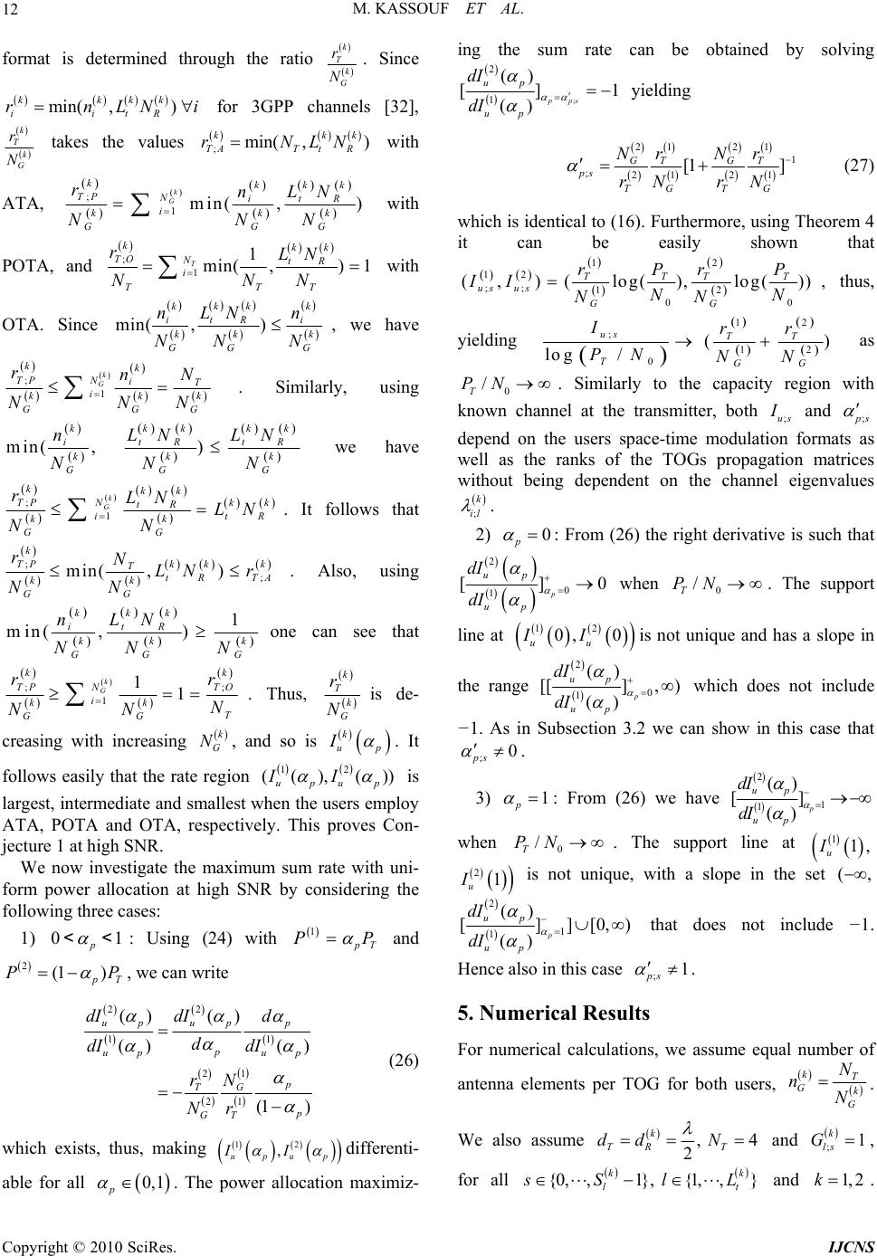

M. KASSOUF ET AL.

12

format is determined through the ratio



k

T

k

G

r

N

. Since

















min( ,)

kkkk

iitR

rnLN



i for 3GPP channels [32],

k

T

k

G

r

N

takes the values













;min( ,)

kk

TATtR

rNLNk

with

ATA,







;1

k

G

k

TP N

kkk

GGG

rnLN

NNN



min( ,)

kk

k

itR

i with

POTA, and

 

;11

min(,)1

T

kkk

TO NtR

i

TTT

rLN

NNN





 with

OTA. Since







min( ,)

kkkk

itR i

kk

GG G

nLN n

NN N

k

, we have



 

;

k

TP

r

1

k

G

k

NiT

i

kk

k

GGG

nN

NN

N





. Similarly, using



min(,

k

i

k

G

n

N

 







)

kk kk

tR tR

kk

GG

LN LN

NN

 we have









;

k

TP

r



1

k

G

kk

NtR

itR

kk

GG

LN LN

NN





. It follows that



 

;

k

TP

r

;

min(,)

kk k

T

tR TA

kk

GG

NLN r

NN



. Also, using





 

1

min



( ,)

kkk

itR

kk k

GG G

nLN

NN N

one can see that



;;



111

k

G

kk

TO

N

i

kk

T

GG

rr

N

NN







TP . Thus,

k

T

k

G

r

Nis de-

creasing with increasing , and so is



k

G

N









k

up

I



. It

follows easily that the rate region









1

(( )

up

2

),()

u p

II



is

largest, intermediate and smallest when the users employ

ATA, POTA and OTA, respectively. This proves Con-

jecture 1 at high SNR.

We now investigate the maximum sum rate with uni-

form power allocation at high SNR by considering the

following three cases:

1) 0

p1



<<: Using (24) with



1

P



p

T

P



and





2(1 )

p

T

P



 P, we can write



22

2

21

(

u

p

T

11

1

())

() ()

(1 )

upp p

up up

p

G

p

GT

d

N

r

Nr





dI dI d

dI dI





 

(26)

which exists, thus, making

















1

,

upu

II



2

p



differenti-

able for all . The power allocation maximiz-

ing the sum rate can be obtained by solving



0, 1

p







;

2

1

()

[]

()

pps

up

dI







1



 yielding



22

11

1

;2121

[1 ]

GG

T

ps

TGTG

NN

rr

rN rN







T

(27)

which is identical to (16). Furthermore, using Theorem 4

it can be easily shown that

 



12

;; 12

00

(,)(log( ),log( ))

TTTT

us us

GG

rPr P

II NN

NN

, thus,

yielding



12

;

12

0

()

log /

us TT

TGG

Irr

PN NN

 as

. Similarly to the capacity region with

known channel at the transmitter, both and

0

/

T

PN

;us

I;ps





depend on the users space-time modulation formats as

well as the ranks of the TOGs propagation matrices

without being dependent on the channel eigenvalues





;

k

il



.

2) 0

p





: From (26) the right derivative is such that









2

0

1

[p

up







]0

dI

dI /PN when . The support

line at

0T







12

0, 0

u

II



uis not unique and has a slope in

the range

2

0

1

()

] ,

()

p

up

dI







[[ which does not include

−1. As in Subsection 3.2 we can show in this case that

)

;ps 0







.

3) 1

p





: From (26) we have



2

1

()

[]

when . The support line at

()

p

up

dI







0/

T

PN











11,

u

I









2

u

I1 is not unique, with a slope in the set (,







2

1

dI

dI 1]

()

[]

()

p

up





[0,)

that does not include −1.

Hence also in this case ;1

ps





.

5. Numerical Results

For numerical calculations, we assume equal number of

antenna elements per TOG for both users,



kT

Gk

G

N

nN

.

We also assume



, 4

2

k

TR T

dd N





 and





;1

k

ls

G



,

for all









{0,,1}, {1,,}

kk

lt

s

SlL  and 1, 2k



.

M. KASSOUF ET AL. 13

We consider the 3GPP spatial channel model of Figure 3

from the standardization document [25] with the follow-

ing parameters for use r :

1, 2k





k

B

S



: The angle of the line-of-sight (LOS) direction be-

tween the base station and user with respect to the

antenna array normal at the transmitter.

k





k

M

S



: The angle of the LOS direction between user

and the base station with respect to the antenna array

normal at the receiver.

k





;

k

Tl



: The mean AOD of cluster . l





;

k

R

l



: The mean AOA of cluster l





;;

ˆk

Tls



: The offset AOD from





;

k

Tl



of path

s

in cluster . l





;;

ˆk

R

ls



: The offset AOA fr om





;

k

R

l



of path

s

in cluster . l

Hence, the AOD and AOA of path

s

in cluster

are given by

l











;;; ;;

ˆ

kkkk

Tls BS TTls

 



l



and,

















;;; ;;

ˆ

kkkk

R

lsMS RlRls





, respectively. For numeri-

cal results, we fix the mean AODs and mean AOAs for

all clusters and .The values of the offset AODs

and AOAs are chosen from the simulation model pre-

sented in [25]. We consider a macrocell environment

with a root mean square (RMS) angle spread of at

the base station and RMS angle spread of at the re-

ceiver with the following characterization:

1, 2k

2o

35o

User one:









11

4, 20o

BS

D



 and





115o

MS



 .

Furthermore, we assume





13

t

L with the following

clustering structure:





1

13S, mean AOD





1

;1 4o

T





and mean AOA





1

;1 38o

R



. The offset AODs and AOAs in degrees are

given by









11

;1;1 ;1;1

ˆˆ

, )(0.2826,4.9447),

TR



(









11

;1;2 ;1;2

ˆˆ

(,

TR



)

and

(1.3594, 23.7899)

 



11

;1;3 ;1;3

ˆˆ

,

TR







3.0389,

.



53.1816





1

22S, mean AOD





1

;2 2o

T





and mean AOA





1

;2 10o

R



. The offset AODs and AOAs in degrees are

given by and

 



11

;2;1 ;2;1

ˆˆ

,0.4984, 8.7224

TR



 





1

;2;2

ˆ,

T



.





1

;2;2

ˆR







4.3101,75.4274





1

31S, mean AOD





1

;3 3o

T





and mean AOA





1

;3 20o

R



 . The offset AOD and AOA in degrees are

given by .

 



11

;3;1 ;3;1

ˆˆ

, 1.0257,17.9492

TR





User two:









22

4, 10o

BS

D



 and





25o

MS



. Fur-

thermore, we assume with the following clus-

tering structure:



22

t

L

Figure 4. The capacity and uniform power allocation rate

regions for two-user orthogonally multiplexed MIMO

broadcast channel with user one employing POTA and user

two employing ATA and 

24

(1) 0.05,5, 510, 510, 510

T

0

P=

ND

6

.

Figure 5. Maximum sum rate for the two-user orthogonally

multiplexed MIMO broadcast channel with user one em-

ploying POTA and user two employing ATA and



24

(1)0.05, 5, 510, 510, 510

T

0

P=

ND

6=0.5. The line ,ps



de-

notes the power allocation (16), (27) that maximizes the sum

rate at high SNR and “x” denote the maximum sum rate

points.





2

12S



, mean AOD





2

;1 3o

T



 and mean AOA





2

;1 17o

R



. The offset AODs and AOAs in degrees are

given by









22

;1;1 ;1;1

ˆˆ

(,)( 0.0894,1.5649)

TR



  and





2

;1;2

ˆ

(,

T







2

;1;2

ˆ)(

R



1.7688,30.9538) .

C

M. KASSOUF ET AL.

14





2

22S, mean AOD





2

;2 4.5o

T



 and mean AOA





2

;2 25o

R





(

. The offset AODs and AOAs in degrees are

given by and

 

22

;2;1 ;2;1

ˆˆ

,)( 0.7431,13.0045)

TR



 





2

;2;2

ˆT



(,





2

;2;2

ˆ) (2.2

R



961,40.1824).

Effect of transmit power: The regions





1

(()

up

I,







2())

up

I



and









12

((), ()

p

CC



)

p

)

are illustrated in Fi-

gure 4 for low, intermediate and high values of 0T

when user one employs POTA and user two employs

ATA. We consider single antenna receivers for both us-

ers, . Figure 4 illustrates the conver-

gence of the capacity and rate regions with 0T to-

ward a rectangle, and that the equality at high SNR of

/PN

/N

 

12

(, )(1,1

RR

NN 

P





1

u

I()

p



and





1()

p

C



is satisfied since









11

ii

rn



, following Theorem 5. However, the rate re-

gions with and without channel knowledge at the trans-

mitter are not equal at high SNR because user two em-

ploys ATA, and while . The corre-

sponding maximum sum rate plots are presented in Fig-

ure 5 with respect to

2, i1,2



2

T

r24

T

N

p



, where “x” denotes the maxi-

mum sum capacity points. We see the convergence at

high SNR of these points toward the line corresponding

to (16), (27) given by ;ps 0.5



.

Effect of space-time modulation: The regions









12

((), ())

upu p

II



and









12

((), ()

p

CC



)

p

are illus-

trated in Figure 6 for users employing space-time modula-

tion formats similar to those of Figure 2. For this example,

the rate region









1

((

up

))

p



2

), ())

u p

II



and capacity region

for OTA coincide. From Figure 6 we

see that the largest capacity and rate regions are obtained

when both users employ ATA, while POTA yields a

smaller region, and the smallest regions are obtained with

OTA. These results reinforce Theorem 1 and Conjecture 1.

 

12

((), (

p

CC



Effect of the number of receive antennas: Figure 7

shows that increasing the number of receive antennas

results in an expansion of the regions





1)

up

I((,



and ((.



2())

up

I



 

12

), ()

pp

CC



)

Effect of multipath propagation: Figure 8 considers

two users employing POTA with single antenna receiv-

ers









12

(, )(1,1

RR

NN )

)

. When the total number of multi-

path components increases from to

 

12

(, )(3,1SS 









12

(, )(6,4)SS (where









12

)(3,1)SS (, is ob-

tained by considering the paths of the first time resolv-

able cluster for user one and the first path for user two),

an expansion of the rate regions is observed, with and

without channel knowledge at the transmitter.

In all figures, we see that the rate region with un-

known channel at the transmitter is contained in the ca-

pacity region for channel knowledge at the transmitter.

6. Conclusions

This paper considered orthogonally multiplexed MIMO

broadcast systems with multi-dimensional space-time

modulation over a deterministic multipath additive

Gaussian channel. We showed that the largest capacity

region is achieved when each user employs all his signal

dimensions on all transmit antennas (which corresponds

to ATA space-time modulation format). The capacity

Figure 6. Two-user orthogonally multiplexed MIMO

broadcast channel with users employing

antennas and different space-time modulation formats

with

(1) (2)

RR

()(1N,N =,1)

(1) 2

T

0

P=

ND .

Figure 7. Two-user orthogonally multiplexed MIMO

broadcast channel with users employing ATA and different

numbers of antenna elements with (1) 40

T

0

P=

ND .

M. KASSOUF ET AL. 15

Figure 8. Two-user orthogonally multiplexed MIMO

broadcast channel with users employing POTA with

and different numbers of propagation

paths with

(1) (2)

RR

()(1N,N =,1)

(1) 7

T

0

P=

ND .

region with informed transmitter and the rate region with

uninformed transmitter using a uniform power allocation

are triangular at low SNR and become rectangular at

high SNR. At high SNR these regions become the same

if and only if all users have full column rank TOG

propagation matrices.

We also investigated the power allocation among users

that maximizes the sum rate, and provided explicit ex-

pressions for such power allocation and the correspond-

ing maximum sum rate at low and high SNR. At high

SNR the power allocation that maximizes the sum capac-

ity is determined by the users’ space-time modulation

format and ranks of the TOGs propagation matrices.

However, when the channel is known (respectively un-

known) at the transmitter the sum rate is maximized at

low SNR by an arbitrary power allocation between users

if they have equal ratios of maximum (respectively av-

erage) eigenvalue to signal space dimensionality; other-

wise it is maximized by allocating the total transmit

power to one user only.

Numerical results for a two-user system using some

examples from the 3GPP spatial channel model show

that the capacity region with an informed transmitter and

the rate region with an uninformed transmitter using a

uniform power allocation expand when the number of

transmit antennas per TOG or the number of receive an-

tennas increases. Furthermore, these numerical results

show that an increase in the number of multipath com-

ponents leads to a rate region expansion with known and

unknown channel at the transmitter.

In this paper we assumed that users do not share signal

dimensions, resulting in an orthogonal multiplexed sys-

tem without interference between users. Future work

will explore systems where some dimensions are shared

between users, and hence interference plays a major role.

Appendix

Proof of Theorem 2

Fix

p



and take T

PWe distinguish the fol-

lowing cases:

0

/N .

0

p





: Since no power is allocated to user one





1(0) 0C



, and (12) yields











22

0CX



  

2

2log(

GT

N

Nr

22

0

)

G

TT

rP

NdD

2

with



X

given in (13).

Hence,

 



2

)(0,)

12

00

(0) (0)

(,

log( /)log( /

T

TT G

r

CC

PN PNN

)

1

p





: Similarly to the previous case, we can show

that

  



1

12

1

00

(1) (1)

(,)(,0)

/ )log(/ )

T

TT G

r

CC

PN PNN



log( .

1

p



0<< : Using (12) we have





()

k

p

C





 



 

0

log( ), leading to

k

kk

kG

T

kkkk

GT

N

rP

XNrNDd





1

0

()

[( ,

log( /)

p

T

C

PN









212

01 12

0

()

)]( ,)

log( /)p

pTT

TGG

Crr

PN NN





<< . Thus, the rate of

change of both





1()

p

C



and





2()

p

C



with

in dB is independent of

0

/

T

PN

p



. In the limit, all the points









01

))] p

p



<<

12

[((),(

p

CC



converge toward the intersec-

tion point of the capacity region boundary with the func-

tion

 



1

2

21

G

T

GT

N

r1

R

Nr

 (28)

in the two-dimensional plane defined by the axes





1

R

and





2

R. The capacity region boundary is characterized

by three points



21

00

(0,log( )),(log( ),0)

TTTT

GG

rPrP

NN

NN and



12

00

(log( ),log( ))

TTT T

GG

rPrP

NN

NN . Since, by definition, the

capacity region is the closure of all the set of achievable

rate pairs, it follows that its boundary contains all the

points

 



2

1

20

(,log( ))

T

G

rP

RN

N

T

with

 



1

10

0log( )

TT

G

rP

RN

N

 ,

C

M. KASSOUF ET AL.

16

and



12

10

(log( ),)

TT

G

rP

R

N

N with

 



2

20

0lo

TT

G

rP

RN

N

 g()

.

Consequently, the limiting capacity region is a rectangle

with lower left corner (0, 0) and upper right corner



12

00

(log( ),log( ))

TTT T

GG

rPrP

NN

NN .

Proof of Theorem 3

The proof of this theorem consists first in deriving the

necessary and sufficient conditions for the equality of





()

k

up

I



and





()

k

p

C



for a given

p



. The necessary

and sufficient conditions for equality of the regions









1

((

up

2

())

p



),

u

II



and









12

((), )CC



(

p)

p

follow by

varying the power allocation

p



in the interval [0, 1].

Assuming a fixed power allocation

p



, we have

Lemma 1:









() ()

kk

p

up

CI







()

k

i

n

if and only if the cor-

responding TOGs propagation matrices have full column

rank and



k

i

r









;

k

ili

k



for all





{1, ,}

k

i

ln

such that

  



1

0

()

kk

kG

ik

T

NP

NND



 = Constant





,1,

G

ii N

k.

(29)

Proof: 1) Assume that









() ()

kk

p

up

IC



. Due to

the uniqueness of the input covariance matrix that maxi-

mizes the average mutual information [36], the covari-

ance matrices associated with





()

k

p

C



and





()

k

up

I



must be equal. Hence, (6) and (7) yield



 





 



1

01;

[]

k

i

k

i

kk

nG

lil kn

T

NP

Ndiag ND







I. (30)

From (30),

  



1

;

0

T

, leading to

full rank TOG propagation matrices. Therefore,

ii

and all eigenmodes in TOG i are active. Fur-

thermore, (30) also leads to

()

kk

G

il k

NP l

NND





k() ()k

rn

  



1

;

0

()

kk

G

il k

T

NP

NND





= Constant





,1,

k

i

ll n.

It follows that









;

k

ili

k



 , and the water-filling con-

stant becomes

  



1

0

(), 1,

kk

kk G

iG

k

T

NP ii N

NND





 

making

  



1

0

()

kk

kG

ik

T

NP

NND



equal for all TOGs.

2) Consider the channel of user with

k





k

G

N TOGs,









k

ii

rnk

and









;

k

il i

k



 for all







1,, i

 k

nl such that

(29) is satisfied. Equation (18) can be written as





  



1

11 0

1

()log[(())]

1log( )

kk

Gi

T

k

G

kk

Nn

kk

N

G

T

up i

kk

il T

G

N

kk

ii

k

i

G

NP

N

IN

NN

n

N



















D

.

Using the arithmetic-geometric inequality [37], we have



  



1

11 0

1

11

( )log[(())]

1log( )

kk

Gi

k

G

kk

Nn

kk

G

T

up i

kk

il

TT

G

N

kk

ii

k

i

G

NP

N

INN

NN

n

N



















D

with equality achieved since

 



1

0

1

()

kk

kG

ik

T

NP

NND



 is

constant for all





1, ,k

G

iN. Hence,



 



 



 



1

10

1

()log[(( ))]

1log( )

k

G

k

G

kk

N

kkk

G

T

up ii

kk

i

T

GT

N

kk

ii

k

i

G

NP

N

In

N

NN

n

N















ND

.(32)

If the channel is known at the transmitter, (29) shows

that there exists a water-filling power allocation where

all eigenmodes are active, and all TOGs contribute to the

overall channel capacity with power



kk

i

T

nP

N allocated

to each TOG , for .Thus, the water-filling

solution leading to the channel capacity results in a con-

stant

i





1, ,k

G

iN

 



 

1

0

()

kk

G

k

T

NP

NND





kk

pi



, leading to



 



11

1

( )log()

kk

Gi

Nn

kk

pp

k

il

G

CN





 k

i



with

 

  



1

11

0

(())

kk

Gi

kk

NnG

ilpik

NP

ND





 

 . Thus,

we have



  



1

0

1(())

k

G

kk

kkk

NG

piii k

TT

NP

n

NNND











and

k

(31)

M. KASSOUF ET AL. 17



 

()

() ()

()()1

10

() ()

() 1

1

()log[(() )]

1log( )

k

G

k

G

Nkk

kkk G

T

pii

kk

i

T

G

N

kk

ii

k

i

G

NP

N

Cn

N

n

N













T

N

ND



(33)

which is similar to (32) and, hence, yielding









() ()

kk

p

up

CI



.

This proves Lemma 1. Now we return to the proof of

Theorem 3.

If









() ()

kk

p

up

CI



for all





0, 1

p



, then (7) and

(19) are identical, and the equality of the rate region









12

), ())

upu p

II



(( and capacity region





1

(()

p

C



,





2

C())

p



is straightforward. If the regions are equal,

then for any value of αp the corresponding point









12

), ())

upu p

II



(( cannot be outside the rectangle with

lower left corner (0, 0) and upper right corner

since

 

12

((), ()

p

CC



)

p









() ()

kk

up p

IC





 

1 2

(), ())

p p

C

 

. In such

case, since (7) and (19) coincide one can easily show that

using the fact

that the capacity region is convex-∩ with

 

12

((), ())

upu p

II







(C





2()

p

C



being monotonically decreasing with p



and





1()

p

C



.

Consequently, the equality of the capacity regions is

equivalent to the equality









()(

kk

)

p

up

CI



 for all





0, 1

p



.

References

[1] E. Telatar, “Capacity of multi-antenna Gaussian chan-

nels,” European Transactions on Telecommunications,

Vol. 10, No. 6, pp. 585–595, November-December 1999.

[2] G. G. Raleigh and J. M. Cioffi, “Spatio-temporal coding

for wireless communication,” IEEE Transactions on Com-

munications, Vol. 46, No. 3, pp. 357–366, March 1998.

[3] G. G. Raleigh and V. K. Jones, “Multivariate modulation

and coding for wireless communication,” IEEE Journal

on Selected Areas in Communications, Vol. 17, No. 5, pp.

851–866, May 1999.

[4] H. Bölcskei, D. Gesbert, and A. J. Paulraj, “On the ca-

pacity of OFDM-based spatial multiplexing systems,”

IEEE Transactions on Communications, Vol. 50, No. 2,

pp. 225–234, February 2002.

[5] W. Bliss, K. W. Forsythe, A. O. Hero III, and A. F.

Yegulalp, “Environmental issues for MIMO capacity,”

IEEE Transactions on Signal Processing, Vol. 50, No. 9,

pp. 2128–2142, September 2002.

[6] C-N. Chuah, D. N. C. Tse, J. M. Kahn, and R. A.

Valenzuela, “Capacity scaling in MIMO wireless systems

under correlated fading,” IEEE Transactions on Informa-

tion Theory, Vol. 48, No. 3, pp. 637–650, March 2002.

[7] T. M. Cover, “Broadcast channels,” IEEE Transactions

on Information Theory, Vol. 18, No. 1, pp. 2–14, January

1972.

[8] T. M. Cover, “Comments on broadcast channels,” IEEE

Transactions on Information Theory, Vol. 44, No. 6, pp.

2524–2530, October 1998.

[9] L. Li and A. J. Goldsmith, “Capacity and optimal re-

source allocation for fading broadcast channels - Part I:

Ergodic capacity,” IEEE Transactions on Information

Theory, Vol. 47, No. 3, pp. 1083–1102, March 2001.

[10] L. Li and A. J. Goldsmith, “Capacity and optimal re-

source allocation for fading broadcast channels - Part II:

Outage capacity,” IEEE Transactions on Information

Theory, Vol. 47, No. 3, pp. 1103–1127, March 2001.

[11] G. Caire and S. Shamai, “On the multiple antenna broad-

cast channel,” in Thirty-Fifth Asilomar Conference on

Signals, Systems and Computers, Vol. 2, pp. 1188–1193,

November 2001.

[12] M. H. M. Costa, “Writing on dirty paper,” IEEE Transac-

tions on Information Theory, Vol. IT-29, No. 3, pp.

439–441, May 1983.

[13] G. Caire and S. Shamai (Shitz), “On the achievable

throughput of a multiantenna Gaussian broadcast chan-

nel,” IEEE Transactions on Information Theory, Vol. 49,

No. 7, pp. 1691–1706, July 2003.

[14] W. Yu and J. M. Cioffi, “Sum capacity of Gaussian vec-

tor broadcast channels,” IEEE Transactions on Information

Theory, Vol. 50, No. 9, pp. 1875–1892, September 2004.

[15] P. Viswanath and D. N. C. Tse, “Sum capacity of the

vector Gaussian broadcast channel and uplink-downlink

duality,” IEEE Transactions on Information Theory, Vol.

49, No. 8, pp. 1912–1921, August 2003.

[16] S. Vishwanath, N. Jindal, and A. Goldsmith, “Duality,

achievable rates and sum-rate capacity of Gaussian

MIMO broadcast channels,” IEEE Transactions on In-

formation Theory, Vol. 49, No. 10, pp. 2658–2668, Oc-

tober 2003.

[17] S.Vishwanath, N. Jindal, and A. Goldsmith, “On the ca-

pacity of multiple input multiple output broadcast chan-

nels,” in IEEE International Conference on Communica-

tions (ICC), Vol. 3, pp. 1444–1450, 2002.

[18] A. Goldsmith, S. A. Ja far, N. Jindal, and S. Vishwanat h,

“Capacity limits of MIMO channels,” IEEE Journal on

Selected Areas in Communications, Vol. 21, No. 5, pp.

684–702, June 2003.

[19] N. Jindal, S. Vishwanath, and A. Goldsmith, “On the

duality of Gaussian multiple-access and broadcast chan-

nels,” IEEE Transactions on Information Theory, Vol. 50,

No. 5, pp. 768–783, May 2004.

[20] H. Weingarten, Y. Steinberg, and S. Shamai (Shitz), “The

capacity region of the Gaussian multiple-input multiple-

output broadcast channel,” IEEE Transactions on Infor-

mation Theory, Vol. 52, No. 9, pp. 3936–3964, Septem-

C

M. KASSOUF ET AL.

18

ber 2006.

[21] M. Sharif and B. Hassibi, “A comparison of time-sharing,

DPC, and beamforming for MIMO broadcast channels

with many users,” IEEE Transactions on Communica-

tions, Vol. 55, No. 1, pp. 11–15, January 2007.

[22] P. Tejera, W. Utschick, J. A. Nossek, and G. Bauch,

“Rate balancing in multiuser MIMO OFDM systems,”

IEEE Transactions on Communications, Vol. 57, No. 5,

pp. 1370–1380, May 2009.

[23] M. Kassouf and H. Leib, “Shannon capacity regions for

orthogonally multiplexed MIMO broadcast channels with

informed transmitters,” in IEEE Wireless Communica-

tions and Networking Conference (WCNC), Vol. 1, pp.

357–362, 2004.

[24] M. Kassouf and H. Leib, “The capacity region of or-

thogonally multiplexed MIMO broadcast channels for

open and closed loop systems,” in Proceedings of Con-

ference on Information Sciences and Systems (CISS),

March 2004.

[25] 3GPP TR 25.996 V 7.0.0, “Spatial channel model for

multiple input multiple output (MIMO) simulations (Re-

lease 7),” Technical specification group radio access

network, 3rd Generation Partnership Project, June 2007.

[26] S. D. Blostein and H. Leib, “Multiple antenna systems:

Their role and impact in future wireless access,” IEEE

Communications Magazine, Vol. 41, No. 7, pp. 94–101,

July 2003.

[27] V. Tarokh, N. Seshadri, and A. R. Calderbank, “Space-

time codes for high data rate wireless communication:

Performance criterion and code construction,” IEEE

Transactions on Information Theory, Vol. 44, No. 2, pp.

744–765, March 1998.

[28] S. M. Alamouti, “A simple transmit diversity technique

for wireless communications,” IEEE Journal on Selected

Areas in Communications, Vol. 16, No. 8, pp. 1451–1458,

October 1998.

[29] R. T. Derryberry, S. D. Gray, D. M. Ionescu, G. Mand-

yam, and B. Raghothaman, “Transmit diversity in 3G

CDMA systems,” IEEE Communications Magazine, Vol.

40, No. 4, pp. 68–75, April 2002.

[30] R. A. Soni and R. M. Buehrer, “On the performance of

open-loop transmit diversity techniques for IS-2000 sys-

tems: A comparative study,” IEEE Transactions on

Wireless Communications, Vol. 3, No. 5, pp. 1602–1615,

September 2004.

[31] T. M. Cover and J. A. Thomas, “Elements of information

theory,” John Wiley & Sons, Inc., 1991.

[32] M. Kassouf and H. Leib, “Information rates for multi-

dimensional modulation over multiple antenna wireless

channels,” European Transactions on Telecommunica-

tions, Vol. 20, No. 5, pp. 463–481, August 2009.

[33] D. A. Harville, “Matrix algebra from a statistician’s per-

spective,” Springer-Verlag New York, Inc., 1997.

[34] R. Webster, Convexity, Oxford University Press INC.,

New York, 1994.

[35] G. J. Foschini and M. J. Gans, “On limits of wireless

communications in a fading environment when using

multiple antennas,” IEEE Wireless Personal Communica-

tions, Vol. 6, No. 3, pp. 311–335, March 1998.

[36] N. Jindal, W. Rhee, S. Vishwanath, S. A. Jafar, and A.

Goldsmith, “Sum power iterative water-filling for mul-

tiantenna Gaussian broadcast channels,” IEEE Transac-

tions on Information Theory, Vol. 51, No. 4, pp.

1570–1580, April 2005.

[37] I. S. Gradshteyn and I. M. Ryzhik, “Table of integrals,

series, and products,” Academic Press, corrected and

enlarged edition, 1980.

Paper Menu >>

Journal Menu >>