Journal of Geographic Information System
Vol. 5 No. 3 (2013) , Article ID: 33285 , 11 pages DOI:10.4236/jgis.2013.53028
Simulation Models and GIS Technology in Environmental Planning and Landscape Management
Department of Industrial and Information Engineering, Second University of Naples, Aversa, Italy
Email: giuliana.lauro@unina2.it
Copyright © 2013 Giuliana Lauro. This is an open access article distributed under the Creative Commons Attribution License, which permits unrestricted use, distribution, and reproduction in any medium, provided the original work is properly cited.
Received March 27, 2013; revised April 29, 2013; accepted May 29, 2013
Keywords: Landscape Ecology; Ecological Network; Dynamical System; GIS Technology
ABSTRACT
Landscape protection that, in the past, has been mainly concerned with its historical, artistic and cultural heritage, follows, nowadays, a systemic methodology that looks at landscape as a high level aggregate of spatial, ecologically different units that interact each other by exchanging energy and materials. Strategic environmental assessment, nowadays, has been adopted in Europe in landscape planning, whose task is to verify the compatibility of territory transformations with respect to their levels of criticality and vulnerability, to evaluate possible future scenarios as consequence of interventions by checking if they are in line with preservation and valorization of environmental. To this aim, we make here a short survey of three different simulation models that can be used as Decision Support System in landscape planning and management. They adopt tools of the Landscape Ecology and are based on GIS (Geographic Information System) technology. The first one consists of a planar graph, the so called ecological graph, whose construction needs the computation of suitable indices of environmental control, proper of Landscape Ecology, such as biodiversity, biological territorial capacity, connectivity. The planar graph, for the considered environmental system, returns a picture of its actual ecological health condition and provides very detailed indications and operational assistance for choosing among possible ecological sustainable interventions. The second one, based on the data used to construct the ecological graph, uses the least-cost path algorithm from GIS technology in order to build an ecological network to prevent and to reduce territorial fragmentation caused by intense processes of urbanisation and industrialisation. At last, an integrated GIS-based approach is developed combining an ecological graph model and a mathematical model based on a nonlinear differential equation of logistic-type with harvesting to perform qualitative predictions on the sustainability of a given territorial plan.
1. Introduction
In recent years, the landscape planning has understood the importance of an “ecological-oriented” analysis of environmental systems more or less affected by degradation and ecological phenomena such as fragmentation and reduction of biodiversity.
To be changed is the very idea of “landscape” which, traditionally identified with that of scenic beauty, has now expanded to indicate all the ways of interactions among nature, environment, land, cultural heritage. The landscape as a “field of knowledge” is the basis for the formulation of the European Landscape Convention, CEP, adopted by the Committee of Ministers of Culture and Environment of the Council of Europe July 19, 2000 and since September 1, 2006, law operating in Italy (Law No. 14 of January 9, 2006). According to this convention “Landscape means a certain portion of territory, as perceived by people, whose character derives from the natural and/or human interrelationships”. In addition to defining the term landscape, Convention determines all the rules for the recognition, protection, preservation, management of the landscape. It is the first international treaty with the objective of promoting the protection, management and planning of European landscapes by promoting European cooperation. The Convention is potentially a real conceptual revolution that brings the community to become the primary stakeholders of the evolution of landscapes in which they live, seen as a cultural strategy for the quality of habitat and also relevant from a social and economic point of view. It encourages citizens to take an active part in decision-making processes that affect the landscape at the local and regional levels. The content of the Convention takes into account the whole of the States Parties and covers natural, rural, urban and suburban areas, including land, inland waters and marine waters. Concerns landscapes that might be considered outstanding, and the landscapes of everyday life, even degraded landscapes (Article 2). The methodologies for successful landscape and environmental planning have been severely challenged when concepts like ecosystems preservation and sustainability have been questioned. The actual challenge is to build transparent and flexible decision-making tools to be used in environmental planning and to embrace a broad range of stakeholder needs together with landscape management requirements. Decision-making process needs the use of interdisciplinary models. A modern approach to the study of landscape shows that it should not be viewed as a mere sum of parts but as a system of relations between the different constituent ecosystems and processes that determine its evolution in time. In the language of Landscape Ecology, this means considering the landscape as a system of ecosystems, ecomosaic, organized in a hierarchical structure and interacting with each other through exchanges of energy and matter, in a fragile equilibrium under dynamic disturbances of both natural and anthrop origin ([1-3]). This research, therefore, uses principles and models proposed by the Landscape Ecology to analyze and assess the environmental quality of a landscape through the identification of appropriate indices of control such as biodiversity, “bioenergy”, connectivity. We refer to the term “bioenergy” as the energy available in the environment, present in different forms like animals, seeds, plants, ruled by suitable metabolic processes. Energy and material “fluxes”, i.e., bioenergy fluxes, through the territory are therefore necessary fundamental processes for biodiversity conservation and capacity of the system to resist at the both natural and anthrop perturbations (resilience). Barriers and surfaces with low permeability to such fluxes hamper the movement of animals, seeds spreading and in general the likelihood of species survival, as they act as external constraints on the natural ecosystem. Modeling these fluxes is therefore necessary to assess the most suitable plan strategies for natural resources conservation management and landscape functionality preservation. A tool in this direction can be represented by the construction of the so called Ecological Graph ([4,5]), as we’ll see in the next Section, that furnishes a picture of landscape ecological health condition and provides very detailed indications and operational assistance to guide toward sustainable interventions. Moreover, this model also allows to determine the status of territorial fragmentation and, hence, to verify the need for ecological network, functional to dispersion of animals and plants. As said, the flows of gens and individuals between populations is essential for the survival of those species that are sensitive to the fragmentation of their habitats, therefore, the loss of ecological connectivity, i.e., the difficulty met by organisms in their movement between resource patches, constitutes a challenge for biodiversity conservation. In the 1980s, the idea of developing national ecological networks surfaced more or less simultaneously in several European countries. The ecological network concept not just prioritizes the conservation of core areas as natural or semi-natural values, but also prioritizes the importance of buffering, maintaining and re-establishing ecological connectivity and nature restoration. Depending on the species and spatial scale of interest the characteristics of an ecological network may differ widely, therefore ecological networks can be identified at continental, regional landscape and local scales. To this aim, in Section 3, we’ll show a procedure ([6,7]), based on the least-cost path algorithm from GIS technology, to build a local ecological network for the National Park of Cilento. Finally, in Section 4, behind the static frame of these two simulation models, we shall propose a mathematical dynamical model in order to investigate the time evolution of the health condition of a territory, namely, of its bioenergy value.
In fact, changes in bioenergy, due to changes in environmental conditions, may produce territorial modifications toward which individual landscapes will tend to move smoothly (attractors) or may produce, instead, critical thresholds that result in radical changes in the state of the ecological system. In this sense, ecological systems are, in fact, said metastable. The investigation on mestability can be performed by means of the study of the equilibrium solutions of suitable differential equations ([8,9]) that model dynamics of the territory’s evolution. The primary objective of these models is to perform qualitative predictions on the sustainability of the territorial planning finding, possibly, critical values of the parameters characterizing the territory itself. In Section 4 we use a nonlinear ordinary differential equation of Logistic-type with Harvesting ([10]), applied to a brownfield, ex-industrial area in the East side of Naples, subject to a Master Plan in the direction of improving the environment and we show the time-evolution trend of its ecological value and the existence of a critical value of a suitable environmental indicator linked to the geometrical setting of barriers to bioenergy fluxes.
2. Ecological Graph
In the modern discipline of Landscape Ecology, the landscape is defined as a heterogeneous land composed of interacting ecosystems that exchange energy and matter, and where natural and anthrop events coexist. In the present model, an environmental system is subdivided in a given number of different landscape-units separated from each other by natural or anthrop barriers. The bioenergy content of each unit may be represented by a circle (node) whose diameter is proportional to the magnitude itself. The barriers can have different degrees of permeability to bioenergy’s flow ([3]). For example, an highway has almost zero value of permeability and determines, hence, a territorial fragmentation. We can represent the various levels of connection, among the units, by arcs whose width is proportional to the bioenergy flux shared among them. The collection of nodes and arcs is called Ecological Graph ([4]) of the environmental system. It can be drawn by means of a software GIS (ArchView 3.x) by using the information, contained in suitable Shape Files furnished by local government, about land uses, presence and connection of road infrastructures (railroads, highways, government and provincial roads), system of water courses (natural and artificial) and administrative subdivision of the various urban territories within the studied landscape. We show, now, how to construct such a graph relative to National Park of Cilento in Campania Region (Italy). Firstly we choose the subdivision in 18 units ([5]) as shown in Figure 1. Let us note that each landscape-unit, in turn, is composed of different ecotopes, i.e., the smallest ecologically homogeneous distinct features in a landscape mapping, with a proper value of Biological Territorial Capacity, BTC, that is the amount of energy (Mcal/m2/year) that they need to dissipate in order to maintain their organizational level.
BTC values can be computed on the basis of a standard classification ([3]), as reported in Table 1, once that it is known the kind of ecotopes.
We now define the bioenergy Mj of the landscape-unit j, j = 1, 2, ··· 18 as:
 (1)
(1)
where Bj is the average value of BTC over all the ecotopes belonging to unit j and  is an environmental index computed as the average between three parameters

Figure 1. Landscape units for the national park of Cilento.

Table 1. Standard classification of BTC values.
kFj, kPj, kDj, each with values in [0, 1], as follows:
 ,
, 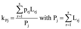

with Pj perimeter of unit j,  perimeter of a circle of area Aj, Lrj the perimeters of the s portions of Pj which have permeability index prj, r = 1, ···, s; nk is the number of ecotopes of BTC of class k among the whole number H of classes present in the unit j. Note that in our case the maximum number of classes is 5 as shown in Table 1.
The first index, kFj, is a parameter related to the shape of the patch borders, since their morphology influences strongly the energy exchanges between the patches themselves. Note that the most jagged is the hedge’s shape the most favorable are the conditions for hiding and reproducing of wildlife.
The second one, kPj, again with the purpose of evaluating energy exchanges, takes into account the permeability of the barriers to energy flux, by following some standard classification ([3]) of values of the permeability parameter as reported in Table 2.
Finally, the third parameter KDj is related to biodiversity, determined by a Shannon entropy value, that takes into account the presence of different ecotopes inside each unit. High values of biodiversity contribute to more stable ecosystems.
Note that, being , we have that the maximum value of bioenergy, Mmax, that a given landscape with n units can produce, will be:
 (2)
(2)
The last environmental indicator needed for evaluating the graph is the bioenergy flux, trough the borders of two consecutive units i and j, whose magnitude is proportional to the width of the link between the nodes of the
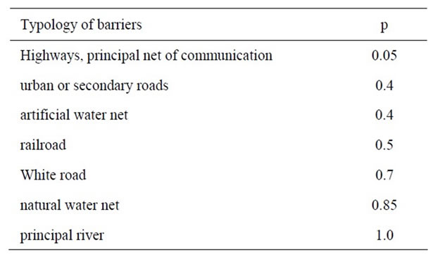
Table 2. Permeability of barriers.
units i and j:
 (3)
(3)
where all the quantities in (3) have already been defined.
For the construction of the ecological graph we have used the software ArcView 3.x of GIS (Geographical Information System).
The shape files, derived from the regional land cover map produced by Campania Region, furnish the information about the land uses, the presence and the connection of road infrastructures (railroads, highways, government and provincial roads), the system of water courses (natural and artificial) and the administrative subdivision of the various urban territories within the studied area.
In Table 3 we have firstly reported the values found, by means of the spreadsheet application of Microsoft Excel, for the bioenergy Mj (normalized to 1), recalling that the diameters of the graph’s nodes are proportional to these magnitudes.
Then, in Table 4 we have reported the values of fluxes Fij (see Equation (3)), normalized to one, between consecutive units, recalling that the width of graph’s arcs are proportional to these values.
The final result of the construction of the Ecological Graph is shown in Figure 2 that exhibits a picture of the actual state of ecological health of this territory.
From the graph of Figure 2 we get, for example, the information that the energetic content of units 1, 14 and 17 (Monti Alburni, Monte Gerbison e Monte Cerviati) is high, hence they represent the territorial portions of greater ecological value and therefore deserve of more attention as they support the entire environmental system. Note from Figure 3 that units 1 and 17 are Special Protection Areas (SPAs), while in unit 14 there is a Site of Community Importance (SCI). Even though, the flux between 1 and 17 is very weak due to the presence of a highway that is not permeable to energy flow. To strengthen this flow it might be possible to carry out structures that allow wildlife to cross above or below the roadway, as studied by the new discipline of Road Ecology. Moreover, the energy content of unit 9 (Monte Centaurino), even if it is characterized by SCI and SPA areas, is very low, as shown by the small size of its node, for the presence of agricultural areas used for annual crops associated with permanent, it would be appropriate to take action for environmental improvement works (hedges of natural vegetation) aimed to increase the level of biodiversity and thus the overall stability of the system. Unit 6 (Valle del Mingardo) is definitely a part of the territory on which it is advisable to aim for improve the system. It is in fact an area characterized by a low value of bioenergy but by a high number of links (5), charac-

Table 3. Bioenergy values of the 18 landscape-units.
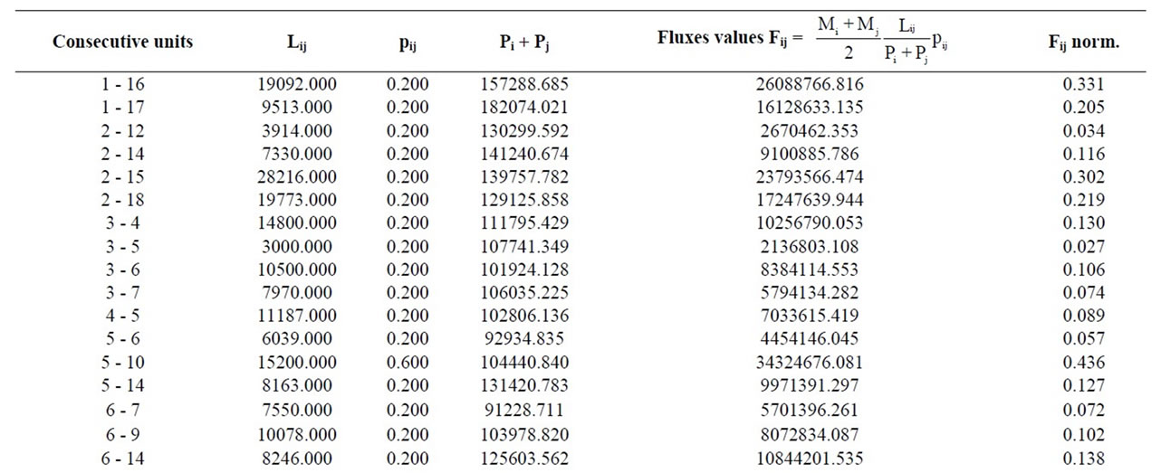

Table 4. Bioenergy fluxes between consecutive landscape-units.
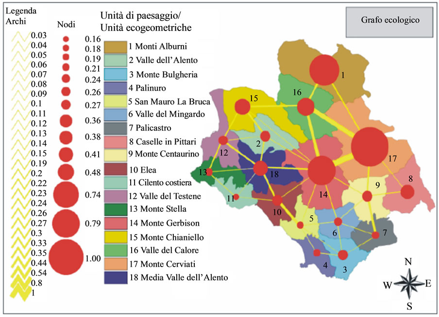
Figure 2. Ecological graph for the national park of Cilento.
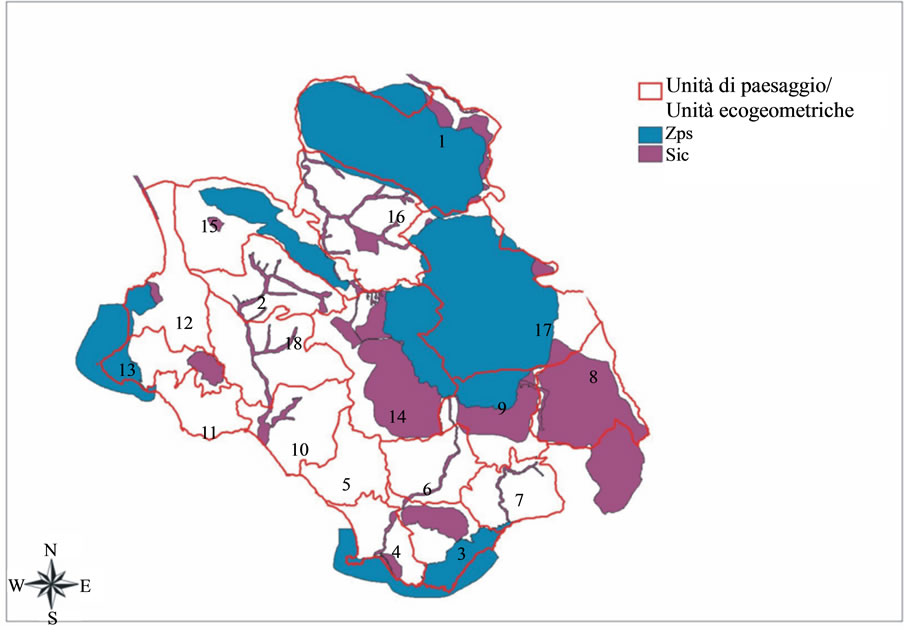
Figure 3. SCI (SIC) and SPAs (ZPS) areas in parco nationale del Cilento.
terized however by weak fluxes, even here, this weakness is linked to the widespread presence of agricultural areas on which to intervene in order to increase the biodiversity. We finally note that as decision-making tool we could match 2 graphs, one representing the actual situation, the second one representing the project solution in line with the intents of a Master Plan if any. The comparison among the graphs of the two sceneries allows, in decisional phase, to judge on the sustainability of the intervention on the area.
3. Ecological Network
As shown by the ecological graph in Figure 2, the studied area suffers of reduction and fragmentation of natural and semi-natural habitats as outcome of agricultural intensification, infrastructure networks and urbanization, even if it is a place of several SCI (Site of Community Importance) and SPAs (Special Protection Areas), as one can see from Figure 3. Recently, eco-regional planning is playing an increasingly important role on the acknowledgment that it is necessary to integrate, from both ecologically and socio-ecologically points of view, the protected areas in the landscape matrix of the entire territory. Hence the origin of ecological networks, characterized by their emphasis on biodiversity conservation at level of region.
The first step consists in creating a resistance map, that is, a map of resistance of the landscape matrix to the mobility of the selected species. In the language of ecological network the zones with the lowest value of resistance play the role of core areas. Then, the least-cost paths linking such areas, i.e., the potential paths that minimize the cost of mobility, are computed ([6]). They represent the corridors of the ecological network that could be adopted as reference information in environmental evaluation of plans and projects in order to reduce as much as possible territorial fragmentation.
The design of corridors for integration in eco-regional planning demands to know the mobility requirements of certain target animal species with rather wide mobility ranges. In our Study Case we have chosen the Peregrine Falcon that lives on the cliffs of the coastal zone of Cilento and is renowned for its speed, reaching over 325 km/h during is hunting. The Peregrine Falcon requires open spaces in order to hunt, he often hunts over open water, marshes, valleys, fields, and tundra, searching for prey either from a high perch or from the air. While its diet consists almost exclusively of medium-sized birds, the Peregrine will occasionally hunt small mammals, small reptiles, or even insects. Hence, we can say that its living space covers all over the Park.
In order to use the least-cost path algorithm, from GIS technology, we need to relate the specific ecological requirements of the chosen species to land uses of the Cilento Park, through a specific parameter called resistance that measures the degree of environmental opposetion to its spread and colonization.
The areas characterized by low value of resistance (resistance equal to zero to the most suitable area) are considered core areas, i.e., natural areas with ecologically high value, for the potential ecological network specific to the species (they could be protected areas too). By using the GIS software used for the graph’s construction we have built the map of resistance ([6]), as shown in Figure 4.
The resistance for the Peregrine Falcon runs from a zero value assigned to bare rocks, cliffs, ponds and meadows, to 60 value for woods, to 90 value for urban areas, rail and road networks. We then apply the PATHMATRIX tool ([7]), an implementation of the least-cost distance algorithm of the GIS software ArcVIEW 3.x, that is able to apply the cost distance algorithm in pair wise fashion among a set of sample locations. PATHMATRIX can also output the length of the least-cost path in geographical distance units. We recall that the least cost path minimizes the sum of resistances along the path (see Figure 5), hence, in our case, it corresponds to the corridor that minimizes the cost of mobility of the target species between the core areas, as shown in Figure 6.
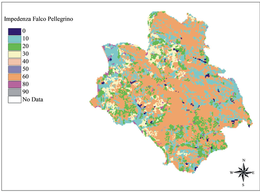
Figure 4. Resistance map for peregrine falcon in the national park of Cilento.

Figure 5. The least cost path minimizes the sum of resistances in going from A to B.
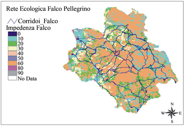
Figure 6. Potential ecological network for peregrine falcon.
The network suggests that along the corridors it would be better to avoid installing equipment in proximity of wetlands, places of wintering of waterfowl and frequented by several species of birds of prey. Also, not installing power lines or wind farms, sources of major impact in the fast flight of Peregrine Falcon. Moreover, rock climbing activity can have negative impact on species whose life is linked to cliffs (nesting, roosting food). Also agricultural activities that impact on the conservation of wildlife could pauperize Falcon’s hunting.
These are some of the considerations coming from a rapid analysis of the ecological network that, hence, can be rightly considered as another decision-support tool in environmental planning and landscape management.

4. Logistic Equation with Harvesting
As said in the Introduction, the Ecological Graph furnishes the actual state of energy exchange in the territory, hence, it would be interesting to investigate the time evolution of energy, starting from the actual settlement, in order to get information on possible future scenarios and check if the trend is toward a sustainable development of the territory or not. This can be made by studying the equilibrium solution of a suitable differential equation that models dynamics of the territory evolution under an ecological point of view. As said in the Introduction, the term “bioenergy” refers to the energy available in the environment, present in different forms like animals, seeds, plants, ruled by suitable metabolic processes, hence, its value must be limited by some carrying-capacity of the given environment. Then, we propose a simulation model based on a logistic-type differential equation ([8]) like that one approximating the evolution of population over time in presence of limited living resources of the environment. Moreover we add a harvesting term in order to simulate the growth of bioenergy over a landscape in spite of the obstacles coming from territory fragmentation.
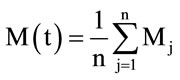
Namely, if we denote by M(t) the average value of the bioenergy (see Formula (2)) over all the n Landscape Units constituting the entire system under study:
 the dynamical simulation model is given by the following nonlinear differential equation
 (4)
(4)
where Mmax, the maximum value of bioenergy the given territory can produce, is given by formula (2) of Section 2 and the connectivity index, c is defined ([8]) by

with V the number of arcs present in the graph constructed for the given territory, Fs, s = 1, ···, V, are the values of energy fluxes given by Formula (3).
In Formula (4), the prime indicates the time derivative, t the time variable, the harvesting term, −hSo, is given by the product of h, the ratio between the sum of the impermeable barrier lengths and the total external perimeter of the territory, and So, the ratio between the sum of the territory surfaces with low values of BTC and the total surface of the system.
Let us note that, from its definition, the connectivity c represents the territorial ability to spread the bioenergy, furnishing, hence, a measure of territorial fragmentation (the flux FS through an impermeable barrier is equal to zero). It plays the role of the constant growth rate as in population dynamics.
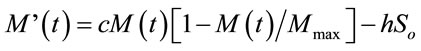
By using the normalized bioenergy , the time evolution equation for M becomes:
M’(t) = cM(t)[1 − M(t)] – hSo (5)
In the application of this model to a Brownfield at the East zone of Naples (Figure 7), subject to a Master Plan in the direction of improving the environment, So will represent the percentage of edified areas, while h will be the ratio between the sum of the perimeters of edified areas and the total perimeter of the area ([9]).
With a similar procedure as before we can construct the ecological graph for this area. We shall not give the details but, instead, we shall provide the main and significant results coming from the mathematical approach based on the study of the equilibrium solutions of Equation (5).
We outline that the mathematical model basic assumption of Equation (5) is that the time evolution of bioenergy will consist of the balance between two quantities with opposite signs. The first one, positive, describes the bioenergy growth by following a logistic law, driven by the connectivity parameter c; the second one, negative, −hSo, the harvesting term, opposes to bioenergy growth due to the presence of barriers related to the edified areas that hamper the flux of energy.
Note that, once subdivided the territory in units as in Section 2, from the relative ecological graphs, as those in Figures 8 and 9, we see that in the project plan the diameters of the nodes, together with the width and the number of the arcs, are increased in line with the planned environmental improvements.
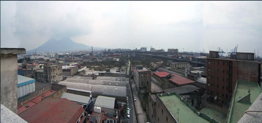
Figure 7. Brownfield-east zone of Naples.
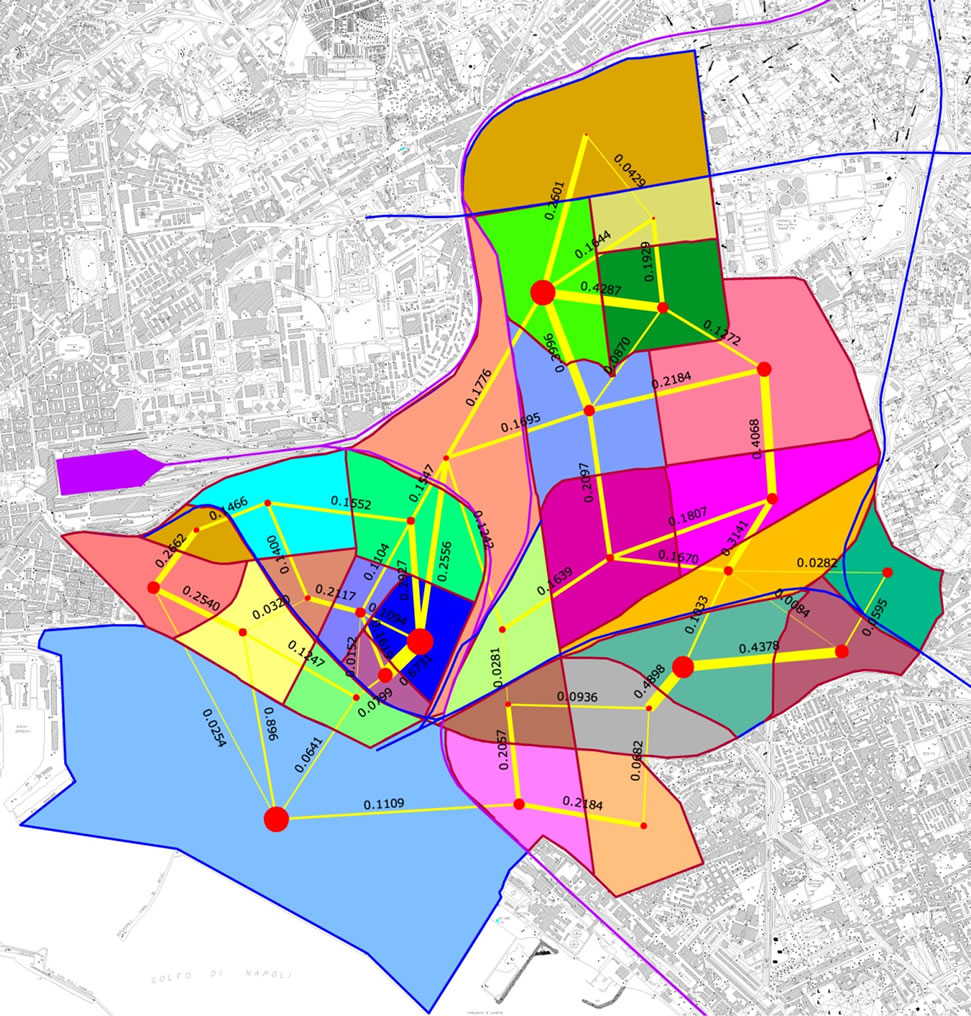
Figure 8. Ecological graph of brownfield actual state.
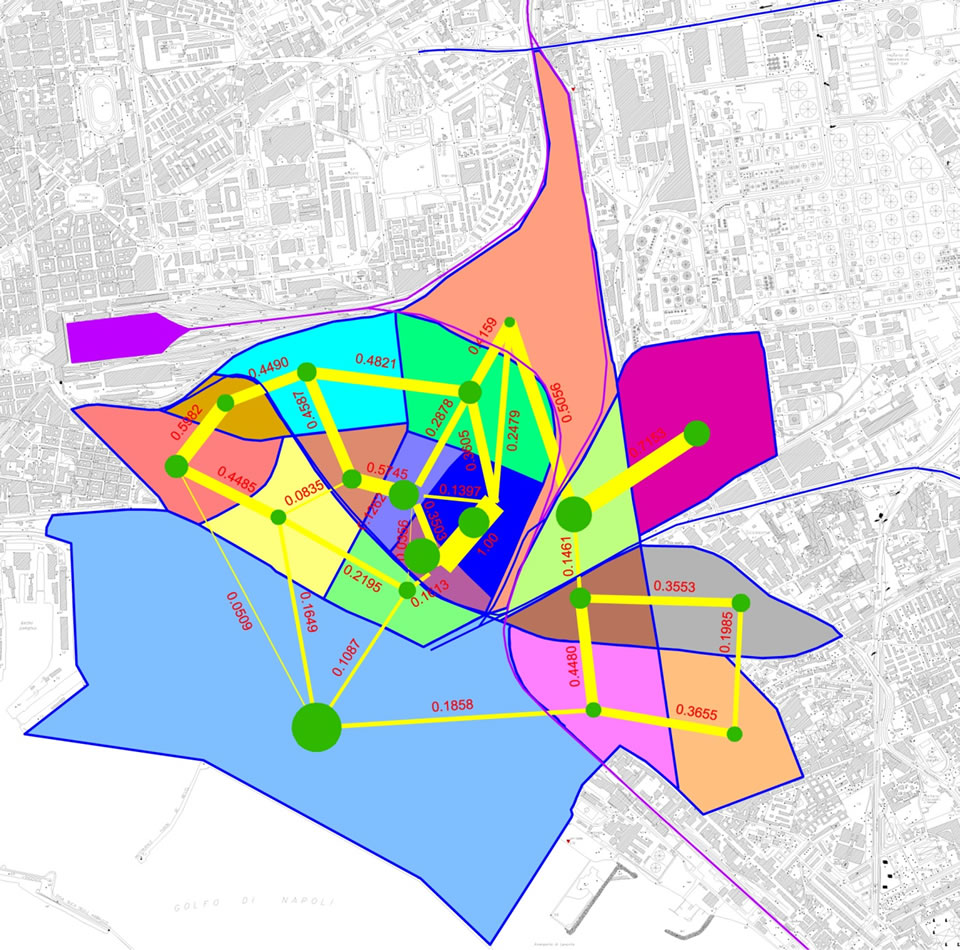
Figure 9. Master plan project ecological graph.
This happens because between the two situations there will be different typologies of intended use of the ground and barriers that will make changes in the analysis and in the calculation of the environmental indices (the Master Plan foresees in fact, among other, the presence of a Urban Park). As a consequence the initial value of M, M(0), as well as the values of c, h and So will change.
If we now turn our attention to the graphs of the solutions ([10]) to the differential Equation (5) of Figure 10, we can see three different possible future sceneries: the first one shows that, starting from the actual state of the area, i.e. with initial value of bioenergy M(0) = 0.048, c = 0.58, h = 0.28, So = 0.79, there is a quick trend to the environmental collapse corresponding to M = 0; in the second one, starting from the project plan, M(0) = 0.086, c = 0.65, h = 0.069, So = 0.66, the value of the bioenergy grows visibly, due to the environmental improvements given by the interventions in line with the Master Plan and tends to a stable good value; the third one furnishes a critical value of the parameter, h = 0.08, at which the system tends to collapse even if it starts from the project value of bioenergy, showing the important role played by the geometrical configuration of impermeable barriers of the buildings.
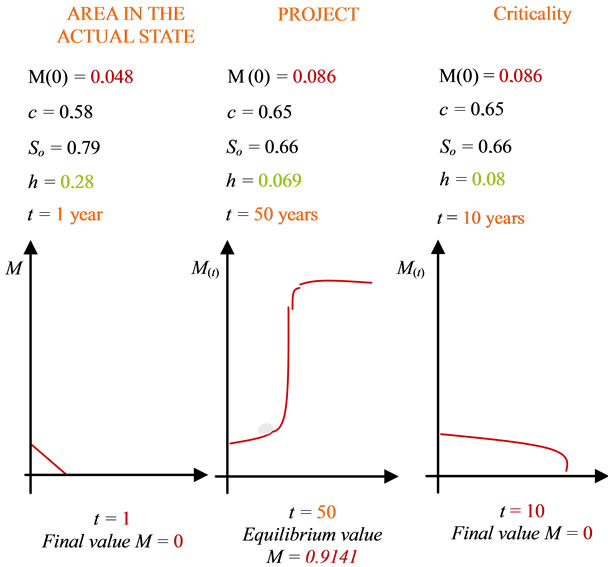
Figure 10. Solution graphs.
We would like to stress that the simple simulation models here presented do not pretend to perform quantitative predictions, but to estimate the goodness of a territorial plan, getting an insight to possible criticalities and hence serving as a decision support in sustainable environmental planning and landscape management.
5. Conclusions
Strategic Environmental Assessment, nowadays, has been adopted in Europe in landscape planning, whose task is to verify the compatibility of territory transformations with respect to their levels of criticality and vulnerability, to evaluate possible future scenarios as consequence of interventions by checking if they are in line with presservation and valorization of environmental quality.
This evaluation must be based, hence, on the knowledge of the mechanisms that rule a territorial transformation. In order to assess the ecological functioning of an environmental system is necessary to single out the energetic contents of the units composing the territory, their connections carrying energy and material fluxes, as well as their breaking points, due to the presence of impermeable barriers, that produce territory fragmentation.
We have presented three different simulation models in the framework of Landscape Ecology, all of them based on GIS technology, which can be used as decision support in environmental planning, such as:
1) Planar graph, the so called ecological graph, whose construction needs the computation of suitable indices of environmental control, proper of Landscape Ecology, such as biodiversity, Biological Territorial Capacity, connectivity. The planar graph for the considered environmental system returns a picture of its actual ecological health conditions and provides very detailed indications and operational assistance to guide toward ecological sustainable interventions.
2) Ecological network, based on the resistance map of target animal species, that gives useful information to prevent and to reduce territorial fragmentation caused by intense processes of urbanisation and industrialisation 3) A mathematical model based on nonlinear differential equation of logistic-type with harvesting used to investigate the time evolution of the ecological value of a given territory, by starting from a given settlement and looking for the trend to consequent future scenarios, hence, furnishing qualitative predictions on the sustainability of a given territorial plan; a recent implementation of this model can be found in [11,12].
These mathematical and GIS interfaced models can help in understanding environment response and dynamic change in time to correctly manage and preserve natural resources; they can represent a powerful decision support to compare effects and impacts of possible alternative future scenarios.
6. Acknowledgements
The author wishes to acknowledge the support given by the Department of Industrial and Information Engineering of the Second University of Naples.
REFERENCES
- R. T. T. Forman, “Land Mosaics. The Ecology of Landscape and Regions,” Cambridge Press, Cambridge, 1995.
- A. Farina A., “Ecologia del Paesaggio,” UTET Libreria, Torino, 2001.
- V. Ingegnoli, “Landscape Ecology: A Widening Foundation,” Springer-Verlag, New York-Berlin, 2002. doi:10.1007/978-3-662-04691-3
- P. Fabbri, “Paesaggio, Pianificazione, Sostenibilità,” Alinea Editrice, Firenze 2003.
- G. Lauro and R. De Martino, “Environmental assessment of the meta-ecosystem Cilento with the tools of Landscape Ecology,” In: C. Gambardella, Ed., Atlante del Cilento, ESI, Napoli, 2009, pp. 533-538.
- G. Lauro and R. De Martino, “The Ecological Network as a Tool for the Protection of Coastal Ecosystems. Workshop: The Mediterranean Coastal Monitoring: Issues and Measure Techniques,” Livorno, 15-16-17 Giugno 2010, Firenze: CNR-IBIMET, pp. 163-170.
- N. Ray, “PATHMATRIX: A Geographical Information System Tool to Compute Effective Distances among Samples,” Molecolar Ecology Notes, Wiley Online Library, 2005.
- G. Lauro, R. Monaco and G. Servente, “A Model for the Evolution of Bioenergy in an Environmental System,” In: T. Ruggeri and M. Sammartino, Eds., Asymptotic Methods in Nonlinear Wave Phenomena, World Scientific, 2007, pp. 96-106.
- G. Lauro and M. Musto, “Simulation Models for Environmental Control,” Proceedings of Sixth EAAE-ENSHA Construction Teachers’ Network Workshop, Mons, 22-24 November 2007, pp. 178-185.
- A. D. Bazykin, “Nonlinear Dynamics of Interacting Populations,” World Scientific, River Edge, 1998.
- F. Gobattoni, R. Pelorosso, G. Lauro, A. Leone and R. Monaco, “A Procedure for Mathematical Analysis of Landscape Evolution and Equilibrium Scenarios Assessment,” Landscape and Urban Planning, Vol. 103, No. 3, 2011, pp. 289-302.
- F. Gobattoni, G. Lauro, R. Monaco and R. Pelorosso, “Mathematical Models in Landscape Ecology: Stability Analysis and Numerical Tests,” Acta Applicandae Mathematicae, Vol. 125, No. 1, 2013, pp. 173-192.