Journal of Geographic Information System
Vol. 4 No. 4 (2012) , Article ID: 22158 , 9 pages DOI:10.4236/jgis.2012.44044
Multi-Temporal Analysis of Remotely Sensed Information Using Wavelets
1Climate and Water Institute, Research Center of Natural Resources, National Institute of Agricultural Technology (CIRN-INTA), Hurlingham, Argentina
2Department of Electronics, Regional Faculty of Buenos Aires, National Technological University (FRBA-UTN), Buenos Aires, Argentina
3National Council of Scientific and Technical Research (CONICET), Buenos Aires, Argentina
Email: acampos@cnia.inta.gov.ar, cdibella@cnia.inta.gov.ar
Received April 27, 2012; revised June 1, 2012; accepted July 5, 2012
Keywords: Land use/cover change; disturbs; vegetation dynamic; MODIS NDVI series; wavelet transform
ABSTRACT
Land cover changes (LCC) are an important component of Global Change. LCC can be described not only by its occurrence, but also by the land cover replacement, causal agent and change duration or recuperation. Nowadays, remote sensing offers the opportunity to assemble reliable time series, however this fails to make a characterization of LCC since the series represents dynamics due to the combination of several processes occurring simultaneously. In this article we proposed an approach to the study of LCC using wavelet transform (WT) and MODIS vegetation time series. Through this work we have demonstrated the capacity of this tool in order to recognize and characterize four different LLC documented in scientific publications, presenting the results divided in frequency scales as interannual, seasonal and rapid changes. The information decomposed in frequency allows the interpretation of each involved process without the interference of others. The uses of WT in an image time series give us the possibility of joining temporal and spatial dimension in a single raster. Layers generated with WT might be used to pattern recognition in LCC and to improve an image classification.
1. Introduction
All Earth’s ecosystems are in a continuous state of change. Transitions from one state to another are originated by natural and/or anthropogenic causes and occurs at several scales of time and space [1-3]. Vegetation transitions are usually catalogued as vegetation phenology when they are driven by the photosynthetic activity through seasons [4], or Land Cover Change (LCC) when the variation of the vegetation is slight or abrupt [1,3]. LCC can be described not only by its occurrence but also by the land cover replacement (e.g. forest to bare land: deforestation, forest to agriculture: agriculturization, grassland to forest: afforestation); causal agent (e.g. cropping, harvesting, natural fires, floodings); and change duration or recuperation. In every case, LCC monitoring is important to understand the vegetation dynamics [4], and, in consequence, to establish relations between policy decisions, regulatory actions or subsequent land use activities [2].
Remote sensing (RS) offers a unique opportunity to collect valuable information to study and understand LCC [1]. Satellite sensor platforms have shown the ability to cover large geographic regions [2], providing multispectral data, with a revisit time ranged from minutes to months, at different spatial resolutions, and available on line for free. According to these intrinsic characteristics, RS have shown its capacity to detect LCC and assemble reliable time series [5-7]. Despite the achievement of regular data, characterizing LCC using RS data is still complex because of the combination of several processes occurring at the same time: seasonal changes, abrupt changes, climate alterations and acquisition errors [8]. The Normalized Difference Vegetation Index (NDVI), calculated from near infrared and red reflectances, was described firstly by Rouse et al. [9] and is widely the most used vegetation index. This index is generally recognized as a good indicator of vegetation activity [6, 10-12] and has been related with several biophysical variables such as: fraction of absorbed photosynthetically active radiation [13,14], leaf area index [14,15], primary production [16,17], among others. Also, NDVI is especially useful in multi temporal datasets because they permit to describe vegetation phenology [5,12,18,19].
In order to detect the occurrence of LCC and to characterize their dynamics, the methodology applied must indentify variability with one temporal scale, while identifying changes with another scale. This means that the methodology must separate changes in ecosystems into three frequency components: seasonal changes (e.g. succession, seasonal precipitation), gradual changes (e.g. interannual temperatures tendencies, land degradation) and abrupt changes (e.g. fire events, flooding, farming) [7]. Signal digital processing offers a wide variety of procedures to detect changes in remotely sensed time series and in monitor vegetation dynamics. The techniques more commonly used are statistical approaches such as principal component analysis [6,11], curve fitting [4,5,20], frequency transformation techniques such as Fourier [12,21], and most recently, Wavelet transform (WT) which has been successfully used to characterize vegetation dynamics [3,22] and expansion-intensification of agriculture [23].
Wavelet transform (WT) is a powerful mathematical tool that has been used since the beginning of the 1980s, but still does not have the diffusion of its precursor: the Fourier transform [24]. The principal advantage of WT is that it has not an unique basis, it is based on a family of functions [25]. As a result, WT has the capacity to disaggregate a signal into its component frequencies (gradual change, seasonal change, etc.), and afterwards describes how each component evolves without interference from the others [26]. Thus, this kind of decomposition introduces the possibility of studying time and frequency domains simultaneously [3,22,27].
The objective of this article is to investigate the potential of time series analysis based on wavelet transform to characterize different LCC at several frequency scales (interannual changes, seasonal changes and rapid changes). We have developed an algorithm capable of applying this transformation to data obtained from MODIS sensor products, allowing us to evaluate a complementary approach to four case studies. These cases were taken from recent publications and they encompass diverse LCC such as fire events, inundations, farming and urbanization from different locations of the globe.
2. Materials and Methods
2.1. Study Sites
In order to embrace different LCC around the globe, we have selected four papers published in the recent years, where localization, region description and vegetation dynamics studies were well documented and published (Table 1).
The four cases encompass: 1) a seasonal inundation in the Mekong Delta where the Tonle Sap Lake increases its area 3 - 6 times in wet seasons [28]; 2) a fire event occurred in August 2006 in the northwest of Spain where almost 930 km2 were burned [29]; 3) a deforestation process n Chaco, Argentina, related to soybean and planted pasture expansion [30]; and 4) a rural to urban conversion in Xi’an region, China [31]. For more details of the studied regions, the mentioned article in each case is recommended (Table 1).
2.2. Satellite Data
In this study, the NDVI time-series have been obtained from the Moderate Resolution Imaging Spectroradiometer (MODIS). MODIS product, MOD13, provides a 16 day NDVI composite, minimizing errors from cloudy days, viewing geometry and atmospheric aerosol presence [19]. Two sources of this product have been used: MODIS Global Subset page (http://daac.ornl. gov/MODIS/modis.shtml) to obtain single pixel ASCII time series; and MODIS WIST (https://wist.echo.nasa.gov/api/) to download complete images in HDF format to obtain time series images (Table 2). In all cases, time-series started on the 18th of February of 2000 and ended on the 26th of June of 2010, spanning 239 measures. We also used two high resolution images from LANDSAT-TM corresponding to the 10th of February of 2001 and the 16th of February of 2009. These LANDSAT-TM images were downloaded from INPE website (http://www.inpe. br/).
2.3. Wavelet Transform Concepts
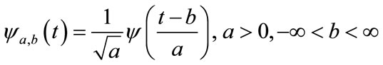
Due to the complex mathematical description of WT, a brief explanation is presented. For further theory and formulae, these publications are recommended: [3,25-27, 32]. The WT is a mathematical tool which decomposes a signal using a family of functions based in a mother
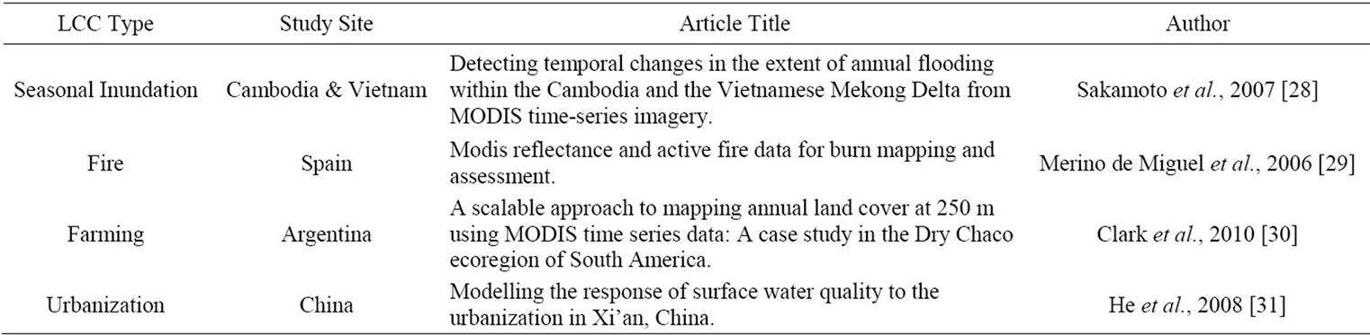
Table 1. Used articles which determine the study regions.
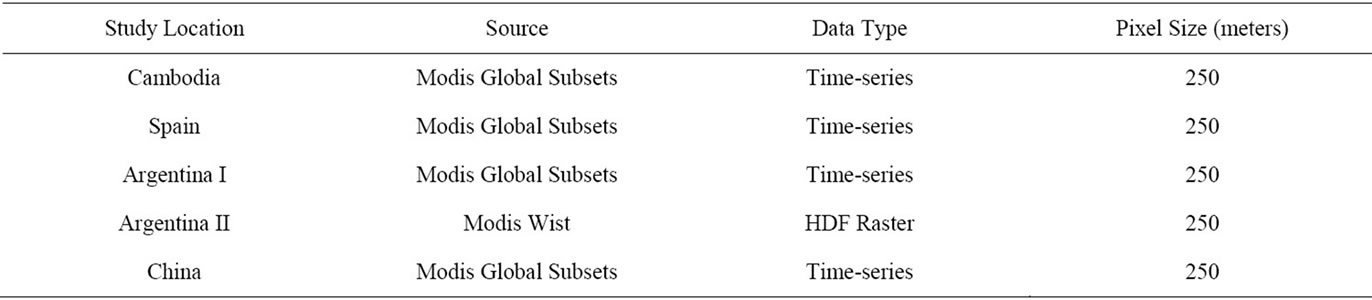
Table 2. Description of the MODIS product acquired for each location.
wavelet [32]:
 (1)
(1)
where  is the family of functions based in dilations and shifts of a mother wavelet
 ;
;  is a coefficient that regulates the dilation and
  adjusts the location. Once the mother wavelet is chosen the WT calculate wavelets coefficients using the following expression:
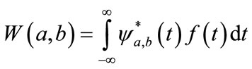 (2)
(2)
where the wavelet coefficients of a function  are represented by
 . For each scale
  and dilation
  a coefficient is calculated. In those cases where the spectral information of
  is similar to the wavelet the coefficient will have higher values [3].
2.3.1. Discrete Wavelet Transform
Discrete wavelet transform (DWT) is a computing efficient implementation of the WT, where scales are based on powers of two (2n). DWT splits a signal into details (D) and approximations (A), using a high frequency pass (HP) and a low pass (LP) frequency pass filters, respectively. Afterwards DWT coefficients are obtained applying a down-sampling with a 2:1 relation to D and A (Figure 1).
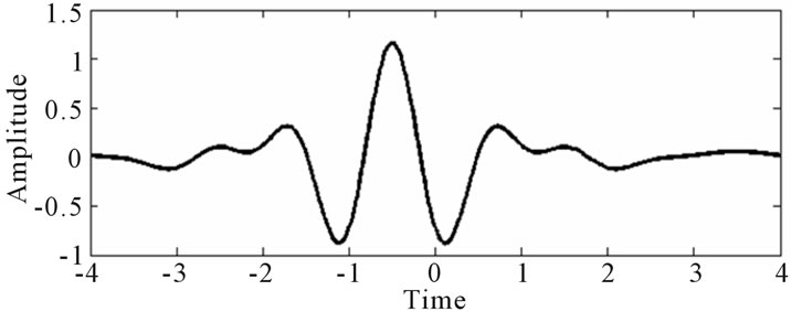
High-pass transfer function is determined by the mother wavelet function ψ, which has to satisfy the admissibility condition and has unitary energy [27]. The low-pass filter is determined by a so called scaling function φ, which is related to some mother wavelets. The selection of a mother wavelet is a difficult task because none of these wavelets has all its properties optimized [26]. Meyer orthogonal discrete wavelet (Figure 2) has been chosen due to its infinitely regularity, its symmetry, and because its mother wavelet permits an exact reconstruction of the original function [33].
2.3.2. Multi-Resolution Analysis
The idea of a multi-resolution analysis (MRA) is the iterative application of the DWT to decompose a signal into several frequencies scales. If we apply the DWT “m” times, the signal f is decomposed into “m + 1” DWT coefficients. After these coefficients are produced, a reconstruction of each frequency scale is made, using up-sampling factors with a 1:2 relation and two reconstruction filters HP’ and LP’ (Figure 3). These reconstruction filters are those which assemble, together with decomposition filters (HP and LP), a quadrature mirror filters system [33].
2.4. NDVI Time-Series Processing
Two types of time-series processing have been made: the
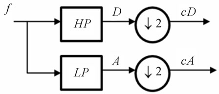
Figure 1. Scheme of a discrete wavelet transform. f is the input signal, HP is the high pass filter, LP is the low-pass filter, A the approximation, D is the detail, cA and cD are the DWT coefficient.
 (a)
(a) (b)
(b)
Figure 2. Wavelets waveforms. (a) Meyer mother wavelet  and (b) its associated scaling function
 .
.
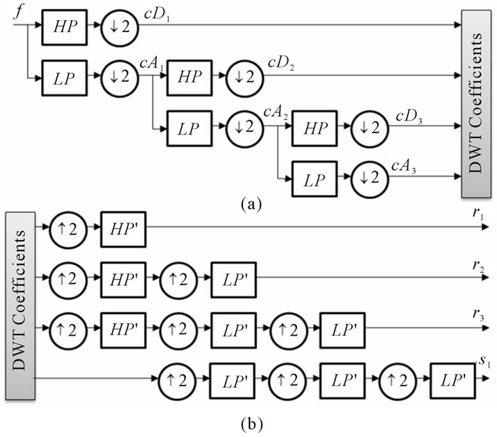
Figure 3. Scheme of wavelet multi-resolution analysis. (a) Decomposition of signal f in three levels (m = 3) producing four scales of WDT coefficients (cD1, cD2, cD3, cA3); (b) Scheme to obtain frequency components, where r1 represent the most rapid changes and s3 represent the slowest changes. HP and LP are the forward high pass and low pass filters, respectively, and HP’ and LP’ are the reconstruction filters.
analysis of two related series per study site and the study of image-time series of a region.
In the first case, two time-series of NDVI from all the locations described previously were processed via DWT. The first signal corresponded to a pixel where a LLC occurs and the second one corresponds to a pixel located nearby of the first one which will provide a control signal. Both signals were decomposed in five levels (m = 4) using the Meyer mother wavelet, where each component meaning is described in Table 3.
In the second case, the images acquired were also attacked by the DWT using five levels and the Meyer mother wavelet. In this topic it is necessary to explain that this study did not perform a bi-dimensional WT. This research decomposed the image time series into five image time series where each one will represent variations at a different frequency scale. As a full representation of image time series will require a video to appreciate the decomposition, we used the time series quadratic sum of some frequency scales to represent the changes. The quadratic sum of a signal can be understood as an indicator of changes, where bigger changes are represented by higher values.
3. Results and Discussion
3.1. Single Point Analysis
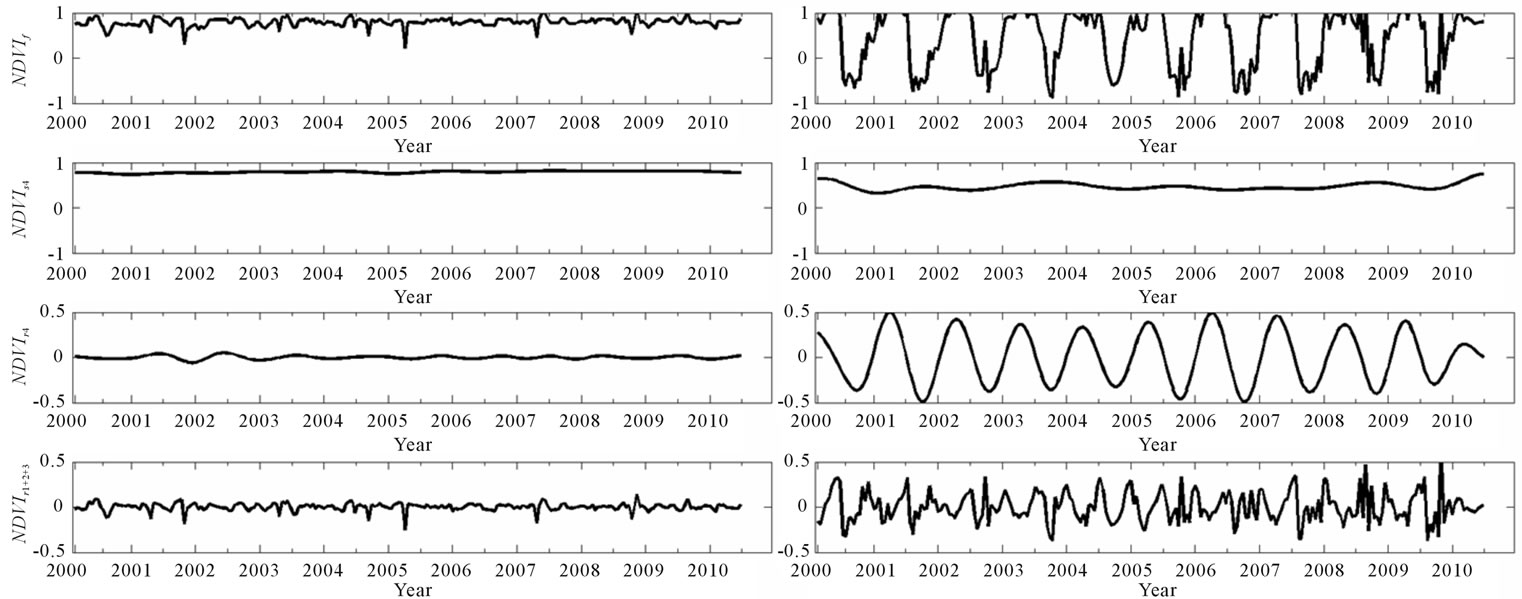
3.1.1. Seasonal Inundation Analysis in Cambodia & Vietnam
Contrast between dry land and floodable land was already
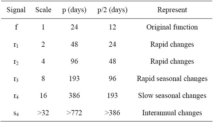
Table 3. Frequency scale description of each signal obtained by MRA, using MOD13 sampling time (T = 16) and the Meyer wavelet, where p is period.
noticeable in the original time-series f, remaining almost constant in the first one and showing cycles in the other (Figures 4(a) and (b)). The NDVIs4 decomposition, which represents the inter-annual changes, showed a mean ± std NDVI value of 0.79 ± 0.021 in the dry land and 0.47 ± 0.078 in the floodable land, implicating a lower photosynthetic activity due to the presence of water in the floodable period. The NDVIr4 reconstruction, which represents slow seasonal changes, had an almost constant value in the dry land and a sinusoidal-like dynamic in the floodable area. This behavior is associated to seasonal variation of NDVI due to inundation, with higher peaks in the first semester and lower values in the second semester, in concordance with the flooding beginning in May-June described by Sakamoto et al. [28]. Finally, the sum of NDVIr1, NDVIr2, and NDVIr3 represented all rapid changes plus rapid seasonal changes in both signals. It was possible to identify that floodable land has more variability than dryland, because of the occurrence of rapid changes originated by the dryland-wetland transition. These variations changed every year and can be related to rainfall variability.
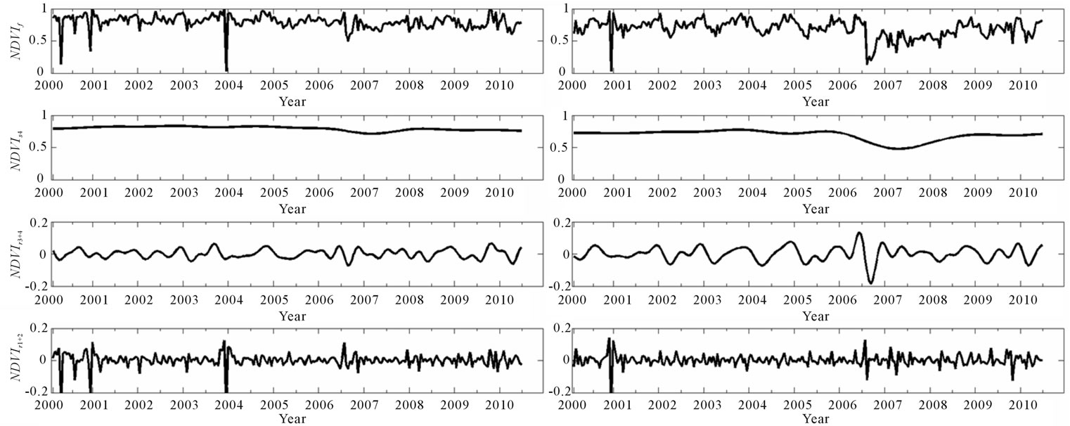
3.1.2. Fire Event Analysis in Spain
Original time series f showed a sudden variation of the NDVI in the year 2006 (Figures 5(a) and (b)) in concordance with a fire event occurred in Galicia in August [29]. Interannual level NDVIs4 illustrates the effect of fire in the location showing a decrease between 2006 and 2007, and vegetation regrowth starting in 2007 and finishing in 2009. Observing the mid-term changes in NDVIr3+4 it is possible to find a discontinuity in the seasonal cycle during 2006 and 2007, denoted by the decrease of higher peaks in the second semester. It is also noticeable the temporal location of the fire-event given by the rapid changes, described in the high frequency scale reconstruction (NDVIr2+1). Other rapids changes showed in NDVIr1+2 are provoked by spurious image acquisition and intraweek changes.
 (a) (b)
Figure 4. Wavelet decomposition of 2000-2010 NDVI time series of dry land (column a) and seasonal floodable land (column b). NDVIf is the original time series, NDVIs4 is the interannual component, NDVIr4 is the slow seasonal component, and NDVIr1+2+3 is the rapid changes component plus rapid seasonal changes.
 (a) (b)
Figure 5. Wavelet decomposition of 2000-2010 NDVI time series of control site (column a) and fire event location (column b). NDVIf is the original time series, NDVIs4 is the interannual component, NDVIr4+3 is the seasonal component, and NDVIr1+2 is the rapid changes component.
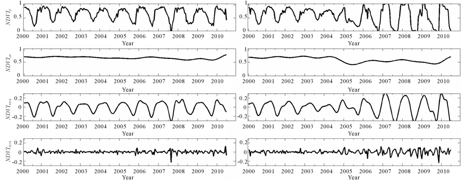
3.1.3. Farming Analysis in Argentina
Differences between the control signal and the farming signal appear since 2005 (Figures 6(a) and (b)). Clark et al. [30] declares that the area was characterized by a rapid deforestation related to soybean and planted pasture expansion between 2002 and 2006. The interannual component NDVIs4 of the agriculturized area showed a decrease of NDVI in 2005, from a mean value of 0.68 to 0.53, meanwhile the control signal remained almost constant. The NDVIr3+4 signal also shows an increment in the peak to peak amplitude due to the replacement of the deciduous forest by crops, meanwhile the maximum amplitude before 2005 was of 0.33, the maximum amplitude after the faming increase to 0.64. In this component it is easy to identify the peaks and the date where they took place, telling us that the forest was replaced by a summer crop. Most rapid changes NDVIr1+2 also increased after 2005 due to the irregular curves of crops alternation.
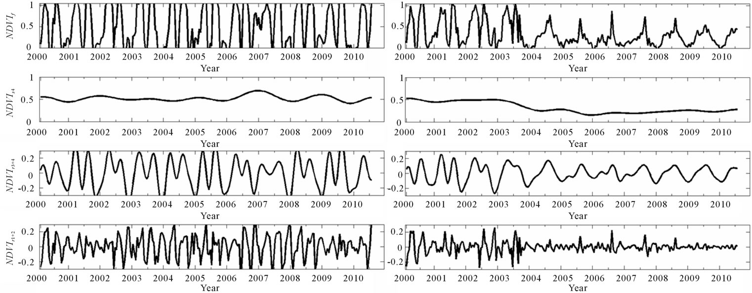
3.1.4. Urbanization Analysis in China
Both original signals do not showed discrepancy until 2004 (Figures 7(a) and (b)) where the original time-series fluctuated from bimodal curves to a sudden decrease in 2004. The NDVIs4 reconstruction showed the interannual
 (a) (b)
Figure 6. Wavelet decomposition of 2000-2010 NDVI time series of control site (column a) and agriculturized land (column b). NDVIf is the original time series, NDVIs4 is the interannual component, NDVIr4+3 is the seasonal component, and NDVIr1+2 is the rapid changes component.
 (a) (b)
Figure 7. Wavelet decomposition of 2000-2010 NDVI time series of control site (column a) and urbanizated location (column b). NDVIf is the original time series, NDVIs4 is the inter-annual component, NDVIr4+3 is the seasonal component, and NDVIr1+2 represent the rapid changes.
change from a mean value of 0.48 to 0.22, as a consequence of the replacement of crops by urbanized structures. The sum NDVIr3+4 reconstructions and the sum NDVIr1+2 also expose a change during from 2004. In the seasonal component the NDVI goes from two crop cultivation per year to a single vegetation peak in August, and the reduction of seasonality is denoted by the decrease of the peak-to-peak magnitude. The rapid changes NDVIr1+2 were also reduced as the urbanization reduced the most rapid changes in vegetation.
3.2. Image Time Series Analysis
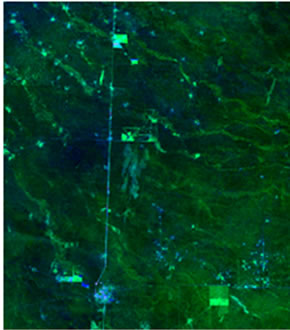
In the frame of this research we also developed a scrpit to process time series analysis from raster data (Section 2.4). As a result, we generated images that joint spatial dimension with temporal analysis. In Figure 8 we represented the ratio between each pixel most rapid changes quadratic sum and the quadratic sum of the original time series. As we have seen previously in item 3.1.3, agriculture has an impact in rapid changes, therefore it was expected that the cultivated places would have a higher quadratic sum (i.e. the higher values in the image). A visual comparison between two high resolution images of the site (where the anthropic activity was noticeable and the energy image was achieved via WT) showed a good recognition of changes. These type of images can be used
 (a)
(a)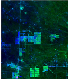 (b)
(b)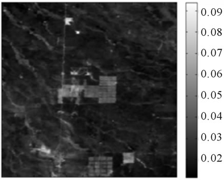 (c)
(c)
Figure 8. Image time series analysis using wavelets. (a) LANDSAT image of 2001-02-10 (Bands 3-4-5 as RGB); (b) LANDSAT image of 2009-02-16 (Bands 3-4-5 as RGB); (c) Energy of most rapid changes (r1) wavelet decomposition in pseudocolor.
as input layers in a classification, because they resume both spatial and temporal information.
4. Conclusions
The study of land cover use and land cover changes, as part of global change, demands the integration of data sources, models and methodologies, and technologies which provide analyzed data according the necessities (e.g. monitoring, alarms, variability research). In response to these requirements, we proposed an approach based in WT. Through this work we had demonstrated the capacity of this tool to study and characterize four different LLC and submitted the results separated in frequency scales (interannual, seasonal and rapid changes). This disaggregated information allowed us to interpret each involved process without the interference of others. The use of WT in image time series gave us the possibility to characterize different change levels in spatial dimension. Layers generated with WT might be used to pattern recognition in LCC and to improve image classification.
It must be said that in this article we worked using NDVI time series, but this tool can be applied to any time series (e.g. leave area index time series, surface temperature time series and others). The use of multiple nature time series might not only describe the LCC at any time scale but also determine its causes.
5. Acknowledgements
Alfredo N. Campos has an INTA post-grade scholarship. This work was supported by INTA (AERN 294001) and by a grant from the InterAmerican Institute for Global Change Research (IAI) CRN2031, which is supported by the US National Science Foundation (Grant GEO045- 2325).
REFERENCES
- P. Coppin, I. Jonckheere, K. Nackaerts, B. Muys and E. Lambin, “Digital Change Detection Methods in Ecosystem Monitoring: A Review,” International Journal of Remote Sensing, Vol. 25, No. 9, 2004, pp. 1565-1596. doi:10.1080/0143116031000101675
- R. Lunetta, J. Knight, J. Ediriwickrema, J. Lyon and L. D. Worthy, “Land-Cover Detection Using Multi-Temporal MODIS NDVI Data,” Remote Sensing of Environment, Vol. 105, No. 2, 2006, pp. 142-154. doi:10.1016/j.rse.2006.06.018
- B. Martínez and M. A. Gilabert, “Vegetation Dynamics from NDVI Time Series Analysis Using the Wavelet Transform,” Remote Sensing of Environment, Vol. 113, No. 9, 2009, pp. 1823-1842. doi:10.1016/j.rse.2009.04.016
- B. A. Bradley, R. W. Jacob, J. F. Hermance and J. F. Mustard, “A Curve Fitting Procedure to Derive InterAnnual Phenologies from Time Series of Noisy Satellite NDVI Data,” Remote Sensing of Environment, Vol. 106, No. 2. 2007, pp. 137-145. doi:10.1016/j.rse.2006.08.002
- P. Jönsson and L. Eklundh, “TIMESAT—A Program for Analyzing Time-Series of Satellite Sensor Data,” Computers & Geosciences, Vol. 30, No. 8, 2004, pp. 833-845. doi:10.1016/j.cageo.2004.05.006
- R. Lasaponara, “On the Use of Principal Component Analysis (PCA) for Evaluating Interannual Vegetation Anomalies from SPOT/VEGETATION NDVI Temporal Series,” Ecological Modelling, Vol. 194, No. 4, 2006, pp. 429-434. doi:10.1016/j.ecolmodel.2005.10.035
- J. Verbesselt, R. Hyndman, G. Newnham and D. Culvenor, “Detecting Trend and Seasonal Changes in Satellite Image Time Series,” Remote Sensing of Environment, Vol. 114, No. 1, 2010, pp. 106-115. doi:10.1016/j.rse.2009.08.014
- D. P. Roy, J. S. Borak, S. Devadiga, R. E. Wolfe, M. Zheng and J. Descloitres, “The MODIS Land Product Quality Assessment Approach,” Remote Sensing of Environment, Vol. 83, No. 1-2, 2002, pp. 62-76. doi:10.1016/S0034-4257(02)00087-1
- J. W. J. Rouse, R. H. Haas, J. A. Schell and D. W. Deering. “Monitoring Vegetation Systems in the Great Plains with ERTS,” 3rd Symposium, NASA SP-351, Washington DC, 1973, pp. 309-317.
- C. J. Tucker and P. J. Sellers, “Satellite Remote Sensing of Primary Production,” International Journal of Remote Sensing, Vol. 7, No. 11, 1986, pp. 1395-1416. doi:10.1080/01431168608948944
- Y. Hirosawa, S. E. Marsh and D. H. Kliman, “Application of Standardized Principal Component Analysis to Land-Cover Characterization Using Multitemporal AVHRR Data,” Remote Sensing of Environment, Vol. 58, No. 3, 1996, pp. 267-281. doi:10.1016/S0034-4257(96)00068-5
- Q. Wang, J. Tenhunen, N. Q. Dinh, M. Reichstein, T. Vesala and P. Keronen, “Similarities in Groundand Satellite-Based NDVI Time Series and Their Relationship to Physiological Activity of a Scots Pine Forest in Finland,” Remote Sensing of Environment, Vol. 93, No. 1-2, 2004, pp. 225-237. doi:10.1016/j.rse.2004.07.006
- C. M. Di Bella, J. M. Paruelo, J. E. Becerra, C. Bacour and F. Baret, “Effect of Senescent Leaves on NDVIBased Estimates of fAPAR: Experimental and Modelling Evidences,” International Journal of Remote Sensing, Vol. 25, No. 23, 2004, pp. 5415-5427. doi:10.1080/01431160412331269724
- G. Posse, M. Oesterheld and C. M. Di Bella, “Landscape, Soil and Meteorological Influences on Canopy Dynamics of Northern Flooding Pampa Grasslands, Argentina,” Applied Vegetation Science, Vol. 8, No. 1, 2005, pp. 49-56. doi:10.1111/j.1654-109X.2005.tb00628.x
- F. Baret, G. Guyot and D. J. Major, “Crop Biomass Evaluation Using Radiometric Measurements,” Photogrammetria, Vol. 43, No. 5, 1989, pp. 241-256. doi:10.1016/0031-8663(89)90001-X
- J. M. Paruelo, M. Oesterheld, C. M. Di Bella, M. Arzadum, J. Lafontaine, M. Cahuepéand and C. M. Rebella, “Estimation of Primary Production of Subhumid Rangelands from Remote Sensing Data,” Applied Vegtation Science, Vol. 3, No. 2, 2000, pp. 189-195. doi:10.2307/1478997
- P. M. Cristiano, G. Posse, C. M. Di Bella and F. R. Jaimes, “Uncertainties in fPAR Estimation of Grass Canopies under Different Stress Situations and Differences in Architecture,” International Journal of Remote Sensing, Vol. 31, No. 15, 2010, pp. 4095-4109. doi:10.1080/01431160903229192
- J. Wang, P. M. Rich and K. P. Price, “Temporal Responses of NDVI to Precipation and Temperature in the Central Great Plains, USA,” International Journal of Remote Sensing, Vol. 24, No. 11, 2003, pp. 2345-2364. doi:10.1080/01431160210154812
- A. Huete, K. Didan, T. Miura, E. P. Rodriguez, X. Gao and L. G. Ferreira, “Overview of the Radiometric and Biophysical Performance of the MODIS Vegetation Indices,” Remote Sensing of the Environment, Vol. 83, No. 1-2, 2002, pp. 195-213. doi:10.1016/S0034-4257(02)00096-2
- X. Zhang, M. Friedl, C. B. Schaaf, A. H. Strahler, J. C. F. Hodges, F. Gao, B. C. Reed and A. Huete, “Monitoring Vegetation Phenology Using MODIS,” Remote Sensing of Environment, Vol. 84, 3, No. 2003, pp. 471-475. doi:10.1016/S0034-4257(02)00135-9
- S. Lhermitte, J. Verbesselt, I. Jonkheere, K. Nackaerts, J. van Aardt, W. W. Verstraeten and P. Coppin, “Hierarchical Image Segmentation Based on Similarity of NDVI Time Series,” Remote Sensing of Environment, Vol. 112, No. 2, 2008, pp. 506-521. doi:10.1016/j.rse.2007.05.018
- T. Sakamoto, M. Yokosawa, H. Toritani, M. Shibayama, N. Ishitsuka and H. Ohno, “A Crop Phenology Detection Method Using Time-Series MODIS Data,” Remote Sensing of Environment, Vol. 96, No. 3-4, 2005, pp. 366-374. doi:10.1016/j.rse.2005.03.008
- G. L. Galford, J. F. Mustard, J. Melillo, A. Gendrin, C. C. Cerri and C. E. P. Cerri, “Wavelet Analysis of MODIS Time Series to Detect Expansion and Intensification of Row-Crop Agriculture in Brazil,” Remote Sensing of Environment, Vol. 112, No. 2, 2008, pp. 576-587. doi:10.1016/j.rse.2007.05.017
- J. F. Kirby, “Which Wavelet Best Reproduces the Fourier Power Spectrum?” Computer & Geosciences, Vol. 31, No. 7, 2005, pp. 846-864. doi:10.1016/j.cageo.2005.01.014
- A. Gupta, S. D. Joshi and S. Prasad, “A New Method of Estimating Wavelet with Desired Features from a Given Signal,” Signal Processing, Vol. 85, No. 1, 2005, pp. 147- 161. doi:10.1016/j.sigpro.2004.09.008
- A. P. Bradley and W. J. Wilson, “On Wavelet Analysis of Auditory Evoked Potentials,” Clinical Neurophysiology, Vol. 115, No. 5, 2004, pp. 1114-1128. doi:10.1016/j.clinph.2003.11.016
- M. O. Domingues, O. Mendes Jr. and A. Mendes da Costa, “On Wavelet Techniques in Atmospheric Sciences,” Advances in Space Research, Vol. 35, No. 5, 2005, pp. 831-842. doi:10.1016/j.asr.2005.02.097
- T. Sakamoto, N. Van Nguyen, A. Kotera, H. Ohno, N. Ishitsuka and M. Yokozawa, “Detecting Temporal Changes in the Extent of Anual Flooding within the Cambodia and the Vietnamese Mekong Delta from MODIS Times-Series Imagery,” Remote Sensing of Environment, Vol. 109, No. 3, pp. 295-313. doi:10.1016/j.rse.2007.01.011
- S. Merino de Miguel, M. Huesca and F. GonzálezAlonso, “Modis Reflectance and Active Fire Data for Burn Mapping and Assessment,” Ecological Modelling, Vol. 221, No. 1, 2010, pp. 67-74. doi:10.1016/j.ecolmodel.2009.09.015
- M. L. Clark, T. M. Aide, H. R. Grau and G. Riner, “A Scalable Approach to Mapping Annual Land Cover at 250 m Using MODIS Time Series Data: A Case Study in the Dry Chaco Ecoregion of South America,” Remote Sensing of the Environment, Vol. 114, No. 11, 2010, pp. 2816-2832. doi:10.1016/j.rse.2010.07.001
- H. He, J. Zhou, Y. Wu, W. Zhang and X. Xie, “Modelling the Response of Surface Water Quality to the Urbanization in Xi’an, China,” Journal of Environmental Management, Vol. 86, No. 4, 2008, pp. 731-749. doi:10.1016/j.jenvman.2006.12.043
- I. Daubechies, “Ten Lectures on Wavelets,” CBMS-NSF Regional Conference Series in Applied Mathematics SIAM, No. 61, Society for Industrial and Applied Mathematics, Philadelphia, 1992.
- MathWorks, “Wavelet Families: Additional Discussion,” MATLAB Help, 2010. http://www.mathworks.com/help/toolbox/wavelet/ug/f8-24282.html