Engineering
Vol. 3 No. 4 (2011) , Article ID: 4600 , 4 pages DOI:10.4236/eng.2011.34045
Comparison between the Isotope Tracking Method and Resistivity Tomography of Earth Rock-Fill Dam Seepage Detection
School of River & Ocean Engineering, Chongqing Jiaotong University, Chongqing, China
E-mail: m.j.zhao@163.com
Received February 2, 2011; revised March 15, 2011; accepted March 23, 2011
Keywords: Earth rock-fill dam, Leakage diagnosis, Isotopes tracing, Resistivity tomography
ABSTRACT
This paper compares the different inversion results of three different earth rock-fill dam models with the actual leakage passages by performing isotope tracing tests and resistivity tomographic tests. The accuracy of the experimental results is evaluated, and the charact-eristics of these two methods are analyzed. As a result, some significant references are offered for earth rock-fill dam’s hidden defects detection. The experimental results show that the leakage and the direction of the seepage can be judged by isotope tracing tests, meanwhile, the degree of the leakage can be confirmed through the determination of the horizontal seepage velocity and the vertical seepage velocity, but it is difficult to properly determine the position of leakage passages and the range of leakage. Relatively speaking, the positions of the leakage passages can be accurately and directly displayed through resistivity tomographic tests. The experiment results show that the resistivity tomographic method is much better than isotope tracing method with regard to earth rock-fill dam’s hidden defects detection, and the resistivity tomographic method expresses much more convenience and much higher precision than isotope tracing method.
1. Introduction
Isotope monitoring technology is an indirect means to infer the seepage characteristics with the help of the different performances of the radioactive tracer when it moves in different parts of the seepage field. Currently, tracer method has already been widely used in the research of oil exploration [1], soil erosion [2-3], groundwater problems [4-5] and so on. Seepage measuring technology by tracer method has been playing an irreplaceable role in quantitatively explaining some difficult problems in major projects. In China, this technology has been successfully applied to detecting the seepage situation of the dam foundation and abutment. Many complex problems in a series of important projects have been solved, such as Xinanjiang hydroelectric power station, Bapanxia hydroelectric power station, Bikou hydroelectric power station, Longyangxia hydroelectric power station, Guangzhou pumped storage power station and Bei Jiang levee.
High density resistivity method is a set of voltage electric prospecting methods which are based on the electric differences between the detected objects underground and the media around them. Steady DC Field underground can be established artificially. With some pre-arranged electrodes, scanning observation is conducted in an order form of scheduled devices and an abundant number of space resistivity variation is studied within a certain range under the ground. Thus, geological problems can be found out and studied. The thought of high density resistivity method has been early considered in the late 1970s and has been firstly proposed by an English doctor named Johansson, and then a system of electrical sounding bias was used as its initial mode which was designed by an English researcher. Shima and Sakayama (1987) firstly used the term “Resistivity Tomography” and proposed the way of inverting explanation. Resistivity tomography technology has been universally applied in foreign countries and has an greatly significant effect in many fields, such as the detection of a hidden danger in the dam [6], the determination of tunnel excavation program [7], karsts probe [8-10], engineering investigation [11], underground mineral deposits prospecting [12-14], detection on erosion distribution of pollutants [15], archaeology [16] and so on. Since the 1980s, electrical prospecting has been rapidly developed and greatly improved in the aspects of method theory and detection techniques. Many theory and application achievements have been gained.
The paper compares the different inversion results with actual leakage passages by isotope tracing and resistivity tomography tests of three different types of earth rockfill dam models. The precision of the results is evaluated and the advantages and disadvantages of two methods are analyzed. Some references can be offered for the detection of hidden defects in earth rock-fill dams.
2. Design of Earth Rock-Fill Dam Model
2.1. Structure of Earth Rock-Fill Dam Model
There are three models of the same size of 3.62 m*3.6 m*1.5 m, and the gradient of the upstream and downstream slope are all 1:1. The plane model of the dam is shown in figure 1.
A hole is reserved in the upstream slope of each dam, through which the tracer can be casted conveniently. While three monitor holes are reserved in the downstream slope, through which the tracer concentration downstream can be monitored conveniently. The pore diameter of these two types of holes is 5 cm, the materials used are PVC piles on which many small holes are reserved to make the water leak conveniently.
The first dam is a homogeneous dam with no core, as is shown in figure 2. The dam is filled of 20% soil, 30% sand and 50% gravel composite. To ensure that the dam body is uniform and dense, and that the compaction degree reaches above 90%, the dam is uniformly tamped by a ramming machine.
The second dam is a dam with a concrete core, as is shown in figure 3. The dam is filled of 15% soil, 30% sand and 55% gravel composite. This second dam is also tamped by a ramming machine to meet the same requirements as the first one.
The third dam is a dam with a soil core, as is shown in figure 4. The core is filled of 20% gravel and 80% clay and its surface is covered by a 15 cm layer of sand. The sand is of well graduation with “30% silt and 30% fine sand and 40% grit”, the dam slope is of well graduation with 100% gravel layer.
2.2. Leakage Passages Setting
As is shown in figure 5, three leakage passages are all reserved at the distance of 106 cm from the left of the core wall for the second and the third dam. The height of these passages are 20 cm, 60 cm, 100 cm respectively. But the first dam is reserved no passages.
3. Model Testing and Results Analysis Based on Isotope Tracing Method
3.1. Basic Principle of Isotope Tracing Method
The basic principle of tracer technology is depicted heafter. After the tracer is determined, it is injected into the filter pile and then the filter pile is put into the checking passage. The water in the filter pile is marked by small amount of the radioactive tracer, the dilution velocity of the tracer is related to the seepage velocity of the groundwater. According to the relationship, the seepage velocity can be worked out. Finally, whether there is seepage field
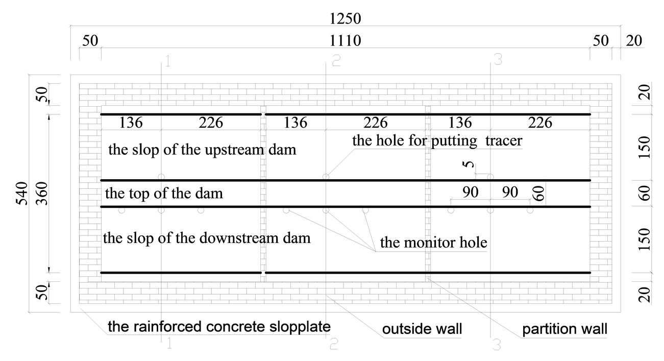
Figure 1. Plain view drawing of the dam model (Unit: cm).
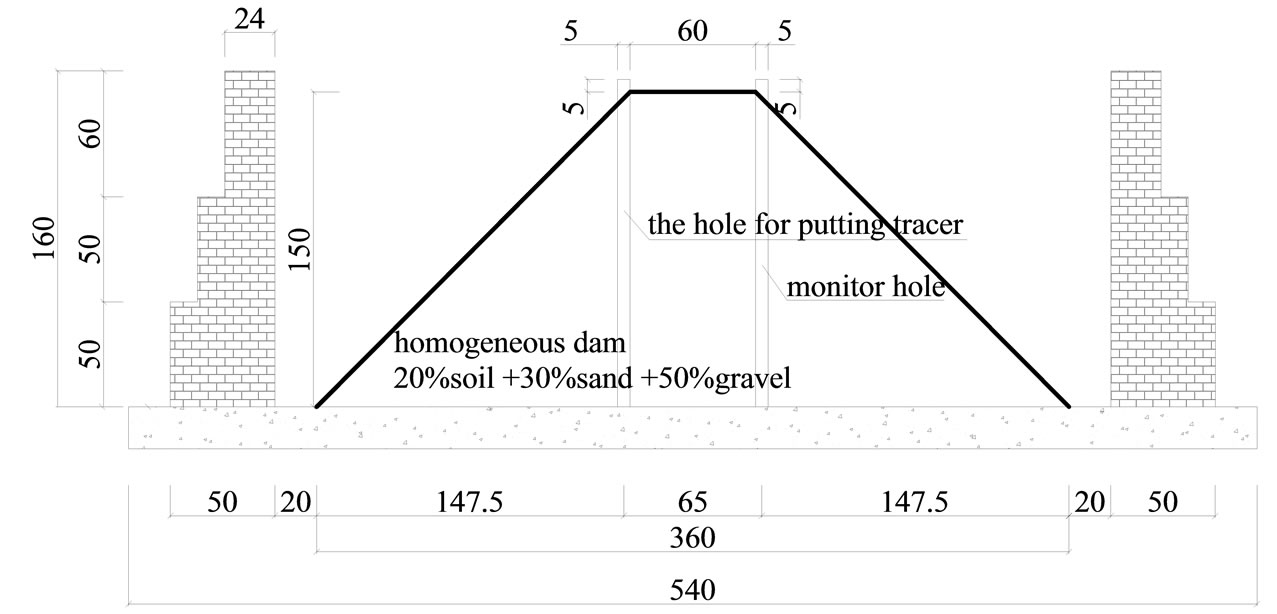
Figure 2. Model of homogeneous dam (Unit: cm).
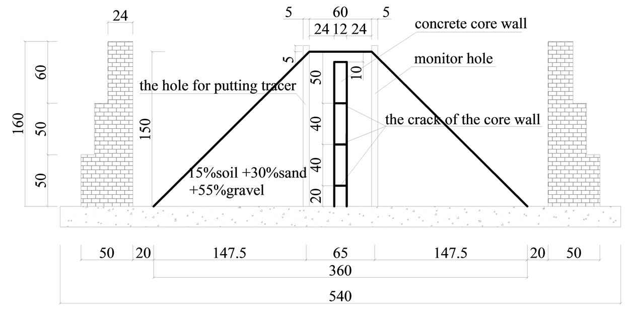
Figure 3. Model of Concrete core dam (Unit: cm).
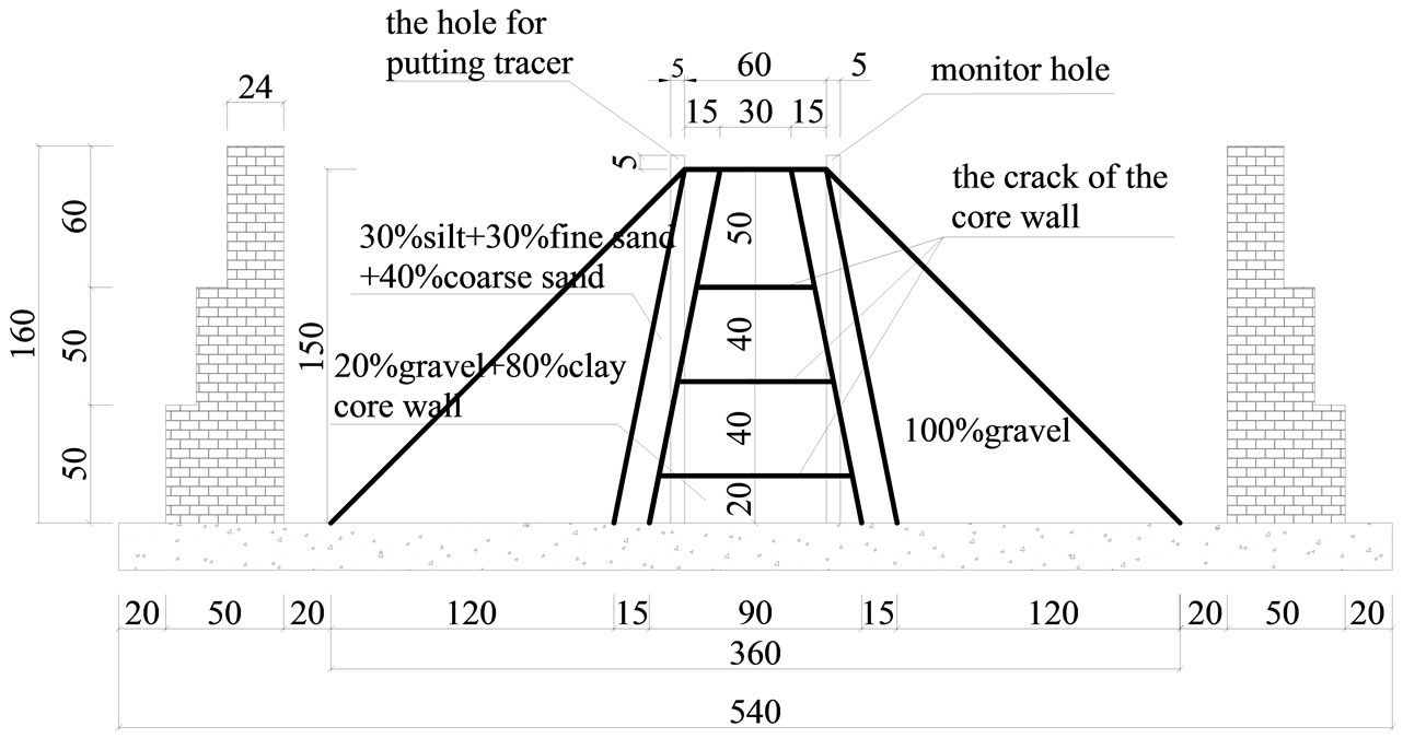
Figure 4. Model of soil core rock-fill dam (Unit: cm).
can be confirmed based on the variation of the seepage velocity. On the available conditions, the work that the tracer is casted and its concentration variation is observed is performed in the same hole, which is called the Single dilution method. In this method, the tracer is adopted to measure the vertical flow in the hole.
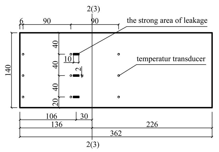
Figure 5. Sketch map of the temperature sensor and leakage passages setting of soil core rock-fill dam and concrete core dam (Unit: cm).
3.2. General Dilution Principle of Artificial Tracer Detecting
It is difficult to meet all the conditions of the spot dilution principle in the process of the practical detection. Therefore the application of the spot dilution technology has been greatly restricted. After extensive study, it is found that the survey still can be conducted by marking the tracer in the whole hole even when there is vertical flow interference in the detected aquifer. If any aquifer has upward vertical flow, the tracer would be put between point A and point B, as is shown in figure 6. The variation of the tracer concentration including that of point A and point B is detected continuously. According to the variation curve the vertical velocity of A and B can be figured out. Supposing that the aquifer corresponding with A and B is uniform distributed, and is of the same water head. As the length of the measured segment is far outweigh the radius of the hole, the influence of the molecular diffusion can be ignored. Further assuming that the concentration at every point on the orthogonal section of holes keeps identical (when the diameter is smaller and the velocity is lower). The distribution of the tracer can not be uniform in the vertical direction. The height of the hole between A and B is h, the radius is r, the velocities of the vertical flow are VA and VB at point A and point B, the total tracer concentration which is detected by detector is written respectively: δ
 (1)
(1)
 (2)
(2)
The recharged sources come from the horizontal flow qA upward the aquifer and the vertical flow at point A from bottom to up. There also are two leakage passages that are qB out of point B and qD to downstream the aquifer. When the tracer flowing from A has reached B, the total water that has come into the diluted water column is mixed with the tracer in the hole. At every point on the orthogonal section, the concentration keep identical, as is shown in figure 7.
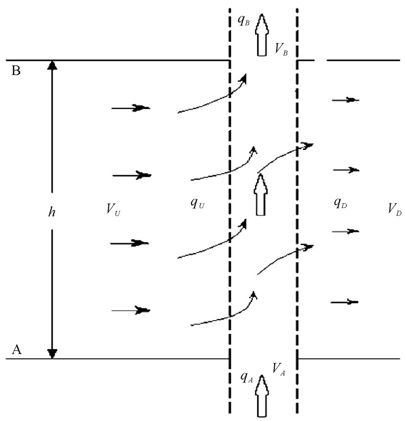
Figure 6. Diagram of the movement of water with vertical flow.
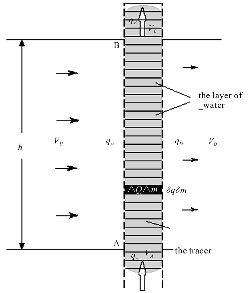
Figure 7. Diagram of the general tracer dilution principle.
3.3. Results and Analysis of Tracer Detecting Test
1) The experiment results of the first dam
The horizontal velocity in the hole can be calculated by using the monitored velocity data. First the monitored conductance data are converted into concentration data, and further converted into relative concentration. The distribution of the concentration in the hole at different time obtained is obtained, as is shown in figure 8.
The horizontal velocity in the hole is calculated by using the general dilution principle of single-hole, and the diagram of the velocity distribution is obtained, as is shown in figure 9.
The distribution curve of the monitored conductance in the hole is sorted out. The changes of the relative concentration curve varying with time can be obtained by using the similar method as in the horizontal velocity calculation, as is shown in figure 10. The peak value of the concentration distribution curve at each time is selected out, and the relationship between the position of the peak value and the cumulated time can be obtained, then the relationship is conducted linear fitting. The linearity of the fitting curve is well, the correlation coefficient is 0.9694, the slope of the line is 0.0723, and the vertical velocity value is 0.0723 cm/s, as is shown in figure 11.
The direction of the flow in the dam is detected by way of the porous tracer method. According to the conductance variation in every drilling hole, the curve of the concentration in the hole varying with time can be obtained. The concentration peak is taken as the direction vector, and the vector multiplying is conducted, then the direction vector of the main seepage is obtained. The angle between the main seepage direction and the vertical line of the second dam is figured out, as is shown in figure 12.
2) The results of the second dam
The experiment process of the second dam is similar
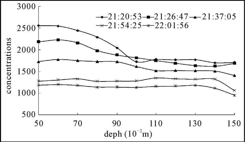
Figure 8. Distribution curve of the concentrations in the hole at different time.
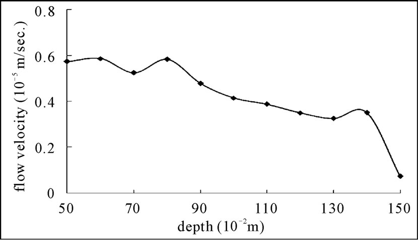
Figure 9. Distribution curve of horizontal flow velocity of the first dam.
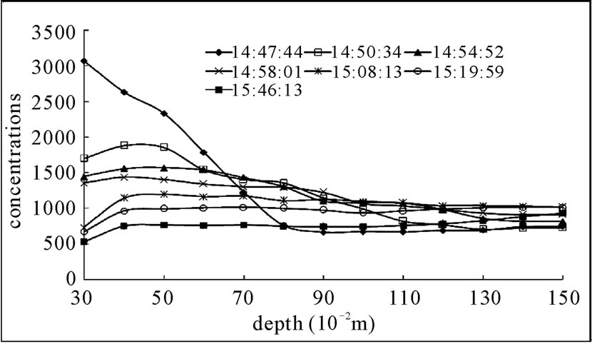
Figure 10. Changing curve of the vertical concentration in the hole.
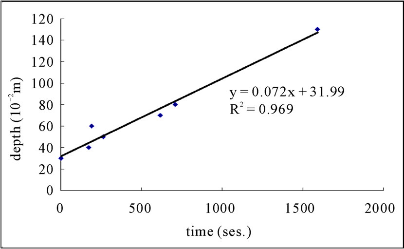
Figure 11. Result of the vertical velocity of the first dam.
to that of the first dam. Firstly, the concentration distribution in the hole at different time is obtained. Then the horizontal velocity in the hole can be calculated by using the general dilution principle of single-hole. Finally, the distribution of the horizontal velocity can be obtained, as is shown in figure 13.
Similarly, the distribution curve of the monitored conductance in the hole is sorted out. The changes of the relative concentration curve varying with time can be obtained by using the similar method as in the horizontal velocity calculation. The peak value of the concentration
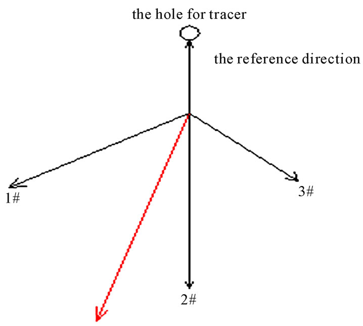
Figure 12. Skech map of the main seepage flow (1#, 2#, 3# represent the tracer concentration of the monitoring hole 1, 2, 3 respectively; The red line is main seepage flow direction; The angle of the other reference direction is 189.3˚).
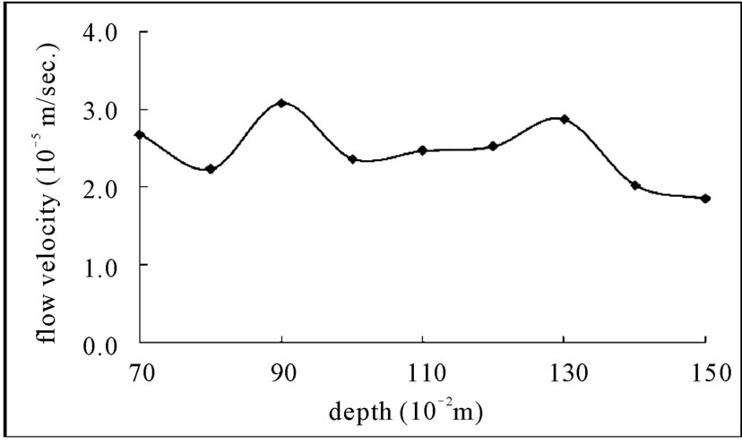
Figure 13. Distribution curve of horizontal flow velocity of the second dam.
distribution curve at each time is selected out, and the relationship between the position of the peak value and the cumulated time can be obtained, then the relationship is conducted linear fitting. The linearity of the fitting curve is well, the correlation coefficient is 0.8653, the slope of the line is 0.1575, and the vertical velocity value is 0.1575 cm/s, as is shown in figure 14.
The vector diagram of the seepage direction of the second dam is similar to that of the first dam, while the angle between the main seepage direction and the vertical line of the dam is 187.1˚.
3) The results of the third dam
The experiment process of the third dam is similar to that of the first and the second dam. Firstly, the concentration distribution in the hole at different time is obtained. Then the horizontal velocity in the hole can be calculated by using the general dilution principle of singlehole. Finally, the distribution of the horizontal velocity can be obtained, as is shown in figure 15.
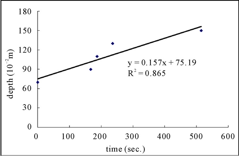
Figure 14. Result of the vertical velocity of the second dam.
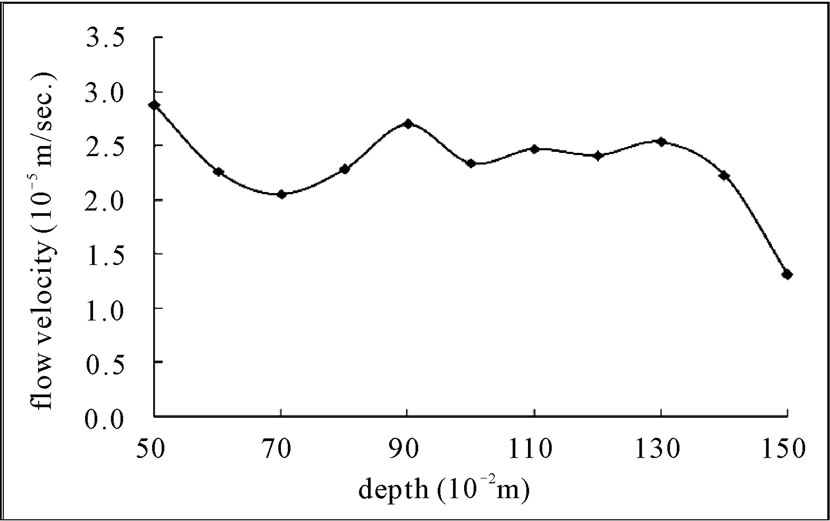
Figure 15. Distribution curve of horizontal flow velocity of the third dam.
Similarly, the distribution curve of the monitored conductance in the hole is sorted out. The changes of the relative concentration curve varying with time can be obtained by using the similar method as in the horizontal velocity calculation. The peak value of the concentration distribution curve at each time is selected out, and the relationship between the position of the peak value and the cumulated time can be obtained, then the relationship is conducted linear fitting. The linearity of the fitting curve is well, the correlation coefficient is 0.8733, the slope of the line is 0.4018, and the vertical velocity value is 0.4018 cm/s, as is shown in figure 16.
The vector diagram of the seepage direction of the second dam is similar to that of the first dam, while the angle between the main seepage direction and the vertical line of the dam is 187.4˚
4. Testing and Results Analysis Based on Resistivity Tomographic Method
4.1. The Principle of Resistivity Tomography
In this experiment, the equipment adopted is the DUK-
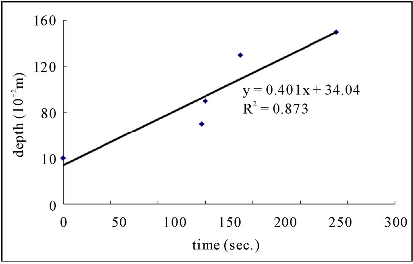
Figure 16. Result of the vertical velocity of the third dam.
2B type electric apparatus which is produced by Geological Instrument Factory of Chongqing of Zhongdi Equipment Group. This system consists of DZD-6 multifunction current electric apparatus and DUK-2 multichannel electrode convertor.
The first survey line is located on the top of the dam, as is shown in figure 17. The second line is located in the downstream slope of the dam, where the height is 1m, as is shown in figure 18. The electrode span of every survey line is 10 cm. As the electrode quantity of the instrument is not enough, each survey line is used for two times. The first dam and the second dam are surveyed in coalition, then the second dam and the third dam are surveyed together.
The basic steps of the test are as follows:
1) The design position of the survey line is accurately measured by a tape measure on the dam model, and then some holes are bored by an impact drill.
2) The tape measure is fastened to the lateral line. Then each electrode is inserted into the dam, and make sure that it contacts well with the dam. The span is 10 cm.
3) The electrodes are connected with the wires. Take note that the relationship between the electrode number and the wire connector is one to one correspondence, and don’t be overlapping and dislocation.
4) Open the instrument, then check whether the voltage of the batteries can meet the survey requirements. Connect the wires with the measuring instrument after confirmation.
5) Attach to the external HV power, and set all measurement parameters.
6) Conduct the ground detecting of the electrodes, and collect data after checking out its good contact with the dam.
7) Exchange the acquisition modes, and collect data respectively. Finally, put up the instrument.
8) The data are imported into a computer, waiting to be handled.
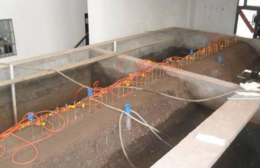
Figure 17. Diagram of the electrodes arrangement of section 1.
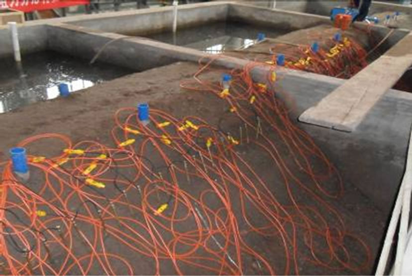
Figure 18. Diagram of the electrodes arrangement of section 2.
4.2. The Experimental Results and Analysis of Resistivity Tomographic Test
1) The regression graph of resistivity tomography of the joint section 1 between dam 1 and dam 2
The regression graph of resistivity tomography of the joint section 1 between the dam 1 and dam 2 is shown in figure 19, which is of inverse echelon distribution. The abscissa represents the horizontal distance between the lateral lines, while the coordinate represents the height of the seepage model, the shade of the color graph illustrates the size of the resistivity. It can be seen from the graph below that the color of the picture on the right is obviously darker than that on the left. The main reason is that the second dam is on the right while the first dam is on the left, the resistance of the dam 2 with a concrete core is obviously higher than that of the dam 1 with no core. The darker part in the middle of the graph represents the concrete partition wall. It is obvious that there is an anomalous area of low resistance in the part near the partition wall on the right of the dam 1. The reason is that there is visible seepage phenomenon at the contact
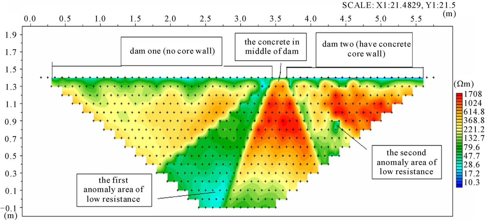
Figure 19. Regression graph of the joint section 1 between dam 1 and dam 2.
site of the dam with the wall, and that is seepage around the dam. There is an anomalous area 2 of low resistance on the left of the dam 2, it is in accordance with the position of the reserved leakage passage.
2) The regression graph of resistivity tomography of the joint Section 2 between dam 1 and dam 2
The regression graph of resistivity tomography of the joint section 1 between dam 1 and dam 2 is shown in figure 20, which is of inverse echelon distribution. The abscissa represents the horizontal distance between the lateral lines, while the coordinate represents the height of the seepage model, the shade of the color graph illustrates the size of the resistivity. It can be seen from the graph below that the darker part in the middle of the graph represents the concrete partition wall. Low resistance area obviously exists in the part near the partition wall on the right of the dam 1. It can be concluded that there are serious seepage phenomenon around the dam 1. Especially, as there is an anomalous area of low resistance on the top of the dam, it also be obtained that there is a seepage passage at the height of 80 cm.The reason is that there are visible seepage phenomenon at the contact site of the dam with the wall, that is seepage around the dam. There is an anomalous area 2 of low resistance on the right of the dam 2, it is in accordance with the position of the reserved leakage passage. The leakage of the seepage passage results in this phenomena.
3) The regression graph of resistivity tomography of the joint section 1 between dam 2 and dam 3
The regression graph of resistivity tomography of the joint Section 1 between dam 2 and dam 3 is shown in figure 21, which is of inverse echelon distribution. The abscissa represents the horizontal distance between the lateral lines, while the coordinate represents the height of the seepage model, the shade of the color graph illustrates the size of the resistivity. It can be seen from the graph below that the color of the picture on the right is obviously darker than that on the left. The main reason is that the second dam is on the left while the third dam is on the right, the resistance of the dam 2 with a concrete core is obviously higher than that of the dam 3 with a soil core. It is obvious that there is still an anomalous area of low resistance in the part near the partition wall on the right of the dam 2. The reason is the seepage around the dam, however it is not more serious than that of the third dam. There is large area of low resistance near the partition wall on the right of the dam 3, which is also because of seepage around the dam, and it is much more serious. Moreover, there exists an anomalous area of low resistance on the top of the dam. The reason is similar to that is narrated in the above. There is an anomalous area 3 of low resistance in the lower left part of the dam 3, which is consistent with the position of the reserved leakage passage.
4) The regression graph of resistivity tomography of the joint Section 2 between dam 2 and dam 3.
The regression graph of resistivity tomography of the joint Section 2 between dam 2 and dam 3 is shown in figure 22, which is of inverse echelon distribution. The abscissa represents the horizontal distance between the lateral lines, while the coordinate represents the height of the seepage model, the shade of the color graph illustrates the size of the resistivity. It can be seen from the graph below that there exists an anomalous area 1 of low resistance near the wall on the left downstream slope of the dam 2. The serious seepage around the dam is the reason, and it is more serious. While on the left of the dam 3, there exists an anomalous area 3 of low resistance,
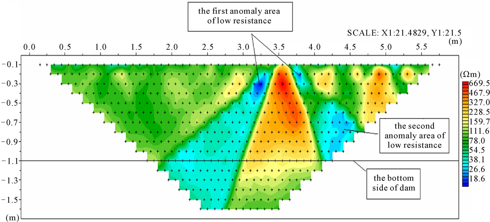
Figure 20. Regression graph of the joint section 2 between dam 1 & dam 2.
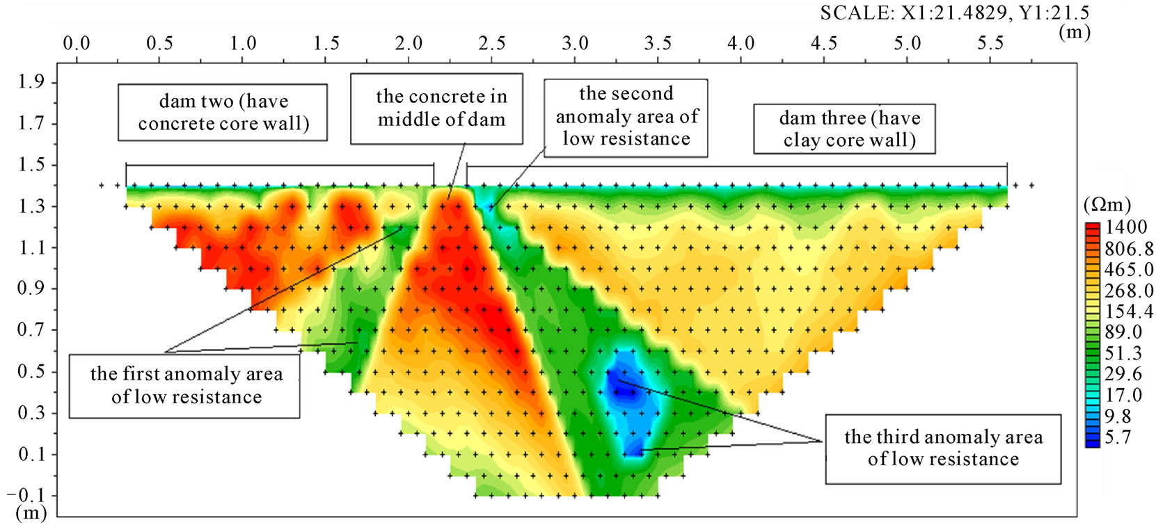
Figure 21. Regression graph of the joint section 1 between dam 2 and dam 3.
and the resistance of other parts is very large, which coin-cides with the position of the reserved leakage passages of the dam 3. There is obviously an anomaly area 2 of low resistance below the bottom line of the dam 3, which is because of the obvious phenomenon of dam foundation seepage.
5. Comparison of Model Testing Results
According to the compared test results of three different types of earth rock-fill dams, Isotope tracing test can be relatively accurate to indicate the position of seepage passages. The seepage parameters in the dam can also be obtained, such as velocities of the horizontal and vertical seepage. Thus this test can provide parameter reference for the dam protection measures. However there are still some disadvantages of the test. Firstly, tracer technology is a kind of damaging detection, which need to punch four holes in the dam. Secondly, the way and quantity of the tracer casting both can bring about data errors. What’s more, the time interval of monitoring can also cause data errors.
Resistivity tomographic test can exactly show the position of seepage passages and the results of the test are very intuitive. But there are also some disadvantages. The span between electrodes can affect the test results and the depth of the monitored profile. In this test, three kinds of electrode arrangement are adopted, which are dipole
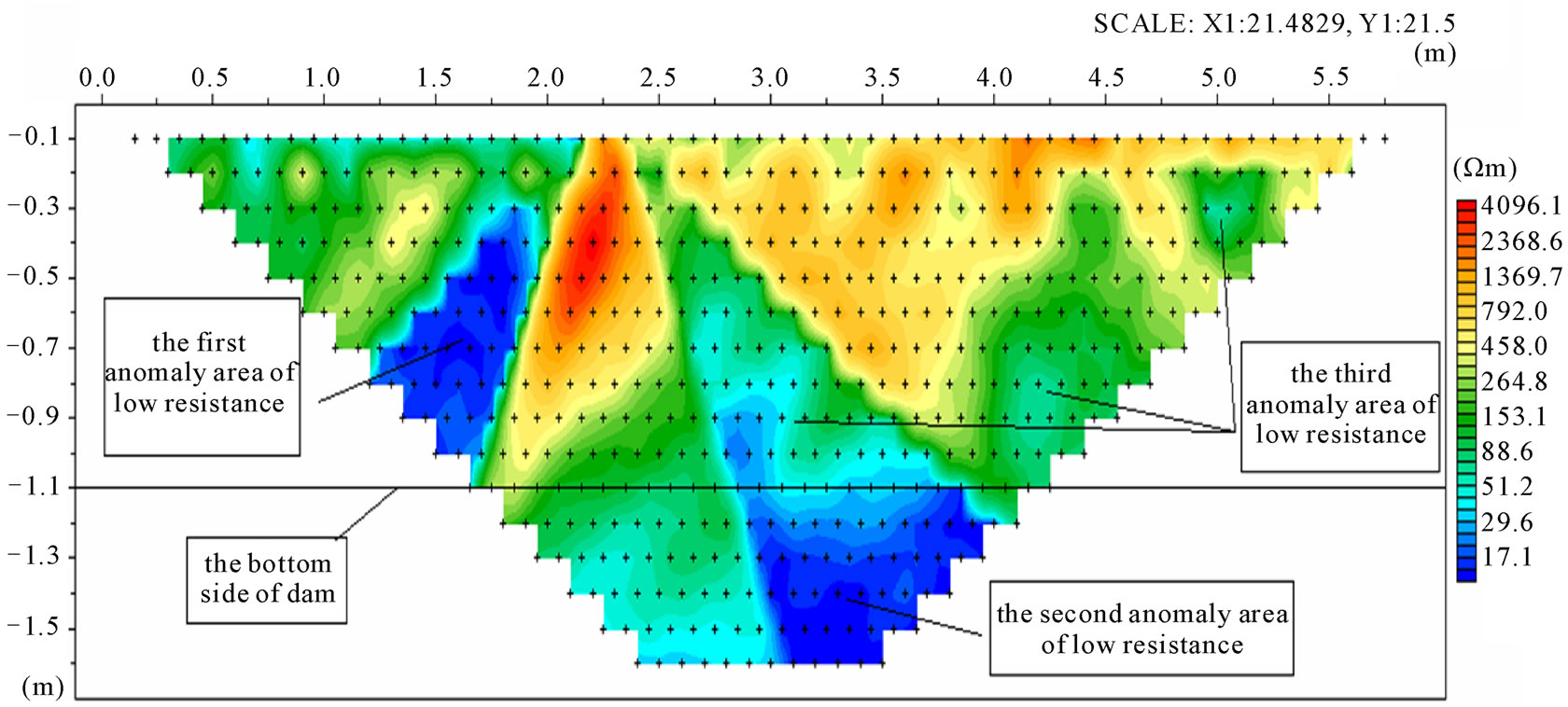
Figure 22. Regression graph of the joint section 2 between dam 2 and dam 3.
arrangement, differential arrangement, and Wenner arrangement. These three ways differ not too much, of which Wenner arrangement and differential arrangement both can reflect the position of seepage passages and the range of seepage. Wenner arrangement has the best diagnostic effect and the first fitting variance is the smallest. In addition, the resistivity tomography test is non-damaging and it can get data without damaging the dam. This test method has achieved good effect in the practical application.
6. Summary
1) Tracer technology is a means of inferring the seepage characteristics with the different performance of the tracer migration in different parts. It is the most direct method of seepage detection and the leakage parameters of the stratum can be directly surveyed without other data. The major disadvantages of this technology are as follows, it is needed to bore a hole in the dam. Besides, because the method surveys the seepage directly, the reason deduction of the leakage and the hidden trouble should be explained by other physical phenomena.
2) The resistivity tomography is a method to find out the geological problems. It is based on the difference of electrical property between the detecting target underground and its surrounding media. The steady current field underground is established in an artificial way. A large number of the space resistivity change is studied in a certain range underground. It can be obtained from the test that the resistivity tomographic technology is the most direct and effective method of seepage survey, and it can also survey the position of the leakage passages and the range of the seepage. The major disadvantages of technology are that the effect of different arrangements and distribution span of the electrode varies greatly.
3) By comparison analysis of this test, it can be concluded that the resistivity tomography is distinctly superior to the temperature field method and the tracer method. The test process of the former is more convenient and of higher precision than the latter two methods.
4) In this test, the local part of the dam is uneven in the model making process, and there also is a problem in the contact with the partition wall between the dams, which can influence the test and lead to data errors. Thus, trying to use homogeneous materials in the process of model making and performing vibration compaction are proposed to reduce the influence of the model itself on the experiment.
5) The tracer test will cause errors because of the interval of the monitoring time and the concentration in the hole. Therefore, trying to keep the concentration up and down the hole identical and trying to shorten the interval of the monitoring time and survey several times are proposed to reduce the data errors.
6) The resistivity tomography test will have errors due to the electrode span and the different arrangement number. Thus, trying to use small span and monitoring by Wenner arrangement are proposed to make the data be of a higher precision.
7. Acknowledgments
This author gratefully acknowledges financial support from the National Natural Science Foundation of China (Grant No. 50779081) and Chongqing Science and Techlogy Plan Project (Grant No: CSTC2007AC -6037).
8. REFERENCES
- Z. Y. Liu and X. F. Song, “Use of Interwell Tracing in Studying the Distribution of Residual Oil in a Reservoir,” Journal of Jianghan Petroleum Institute, In Chinese, Vol. 21, No. 4, 1999, pp. 76-78.
- W. Song, J. L. Liu and M. Y. Yang, “Study on Erosion Process by the REE Tracer Method,” Advances in Water Science, Vol. 15, No. 2, 2004, pp. 197-201.
- K. Ma and Z. Q. Wang, “Summary of Tracer Method on Studies of Soil Erosion,” Research of Soil and Water Conservation, Vol. 9, No. 4, 2002, pp. 90-95.
- L. X. Yao, W. F. Chang and Y. Han, “Application of the Tracer Method of Hydraulic Engineering in the Survey Leakage,” Yellow River, No. 10, 2009, pp. 98-99.
- J. S. Chen, H. Z. Dong and Z. C. Fan, “Nature Tracer Method for Studying Leakage Pathway of By-Pass Dam Abutment of Xiaolangdi Reservoir,” Jourmal of Yangze River Scientific Research Institute, Vol. 21, No. 2, 2004, pp. 14-17.
- D. Yu, M. J. Zhao and J. G. Yang, “Experimental Research of Electrical Resistivity Tomography Detection Method in Leakage Passage of Earth Rock-Fill Dam,” Journal of Chongqing Jiaotong University (Natural Science), Vol. 29, No. 2, 2010, pp. 224-226.
- D. Li and K. H. Xiao, “High Density Electrical Resistance Exploration in the Tiefengshan Tunnel,” Chinese Journal of Engineering Geophysics, Vol. 3, No. 3, 2006, pp. 197-200.
- L. G. Zhang and J. Liu, “Application of High Density Resistivity Method to the Exploration of Karst Cave under Roadbed,” Soil Engineering and Foundation, Vol. 20, No. 5, 2006, pp. 69-71.
- S. K. Huang and Y. F. Ouyang, “Application of High Density Electrical Method to Karst Exploration,” Chinese Journal of Engineering Geophysics, No. 6, Vol. 17, 2009, pp. 720-723.
- X. Y. Lei, Z. W. Li and J. P. Zhe, “Research of High Density Resistivity in the Prospecting of the Soil Cave, Area of Coal Pits and Karst,” Progress in Geophysics, Vol. 24, No. 1, 2009, pp. 340-347.
- J. H. Deng, W. B. Li and D. S. Zhang, “Application of High Density Resistivity Method in Slope Investigation for Highway,” Geotechnical Engineering Technique, Vol. 22, No. 1, 2008, pp. 27-30, 35.
- Y. K. Men, G. H. Fan and A. L. Shao, “The Study of Integrated Detection Method to the Mined-Out Areas in Open Pit Iron Mine and Its Application,” Metal Mine, No. 5, 2010, pp. 124-127.
- S. P. Li, “The Application of the High Density Resistivity Method to the Prospecting for Bauxite Deposits,” Geophysical and Geochemical Exploration, Vol. 33, No. 1, 2009, pp. 8-9, 15.
- P. S. Zhang, J. S. Wu and S. D. Liu, “Testing with High Density Resistivity Method in Prevention and Cure for Mine Water Disaster and Its Applied Effect,” Chinese Journal of Coal Society, Vol. 13, No. 2, 2007, pp. 165-169.
- H. L. Liu, Q. Y. Zhou and H. Q. Wu, “Laboratorial Monitoring of the LNAPL Contamination Process Using Electrical Resistivity Tomography,” Chinese Journal of Geophysics, Vol. 51, No. 4, 2008, pp. 1246-1254.
- Y. J. Su, X. B. Wang and J. Q. Luo, “The Ahaeological Application of Resistivity Tomography Method to Ditch Exploration on Sanxingdui Site,” Progress in Geophsics, Vol. 22, No. 1, 2007, pp. 268-272.