Materials Sciences and Applications
Vol.06 No.11(2015), Article ID:61370,21 pages
10.4236/msa.2015.611103
Composite Materials Damage Modeling Based on Dielectric Properties
Rassel Raihan1*, Fazle Rabbi2, Vamsee Vadlamudi2, Kenneth Reifsnider1
1University of Texas at Arlington, Arlington, USA
2University of South Carolina, Columbia, USA

Copyright © 2015 by authors and Scientific Research Publishing Inc.
This work is licensed under the Creative Commons Attribution International License (CC BY).


Received 22 September 2015; accepted 20 November 2015; published 23 November 2015

ABSTRACT
Composite materials, by nature, are universally dielectric. The distribution of the phases, including voids and cracks, has a major influence on the dielectric properties of the composite materials. The dielectric relaxation behavior measured by Broadband Dielectric Spectroscopy (BbDS) is often caused by interfacial polarization, which is known as Maxwell-Wagner-Sillars polarization that develops because of the heterogeneity of the composite materials. A prominent mechanism in the low frequency range is driven by charge accumulation at the interphases between different constituent phases. In our previous work, we observed in-situ changes in dielectric behavior during static tensile testing, and also studied the effects of applied mechanical and ambient environments on composite material damage states based on the evaluation of dielectric spectral analysis parameters. In the present work, a two dimensional conformal computational model was developed using a COMSOLTM multi-physics module to interpret the effective dielectric behavior of the resulting composite as a function of applied frequency spectra, especially the effects of volume fraction, the distribution of the defects inside of the material volume, and the influence of the permittivity and Ohmic conductivity of the host materials and defects.
Keywords:
Polymer Matrix Composite Materials, Dielectric Properties, Degradation of Composite Materials, Broadband Dielectric Spectroscopy (BbDS)

1. Introduction
The applications of composite materials are now widespread because of their various advantages over conventional isotropic materials. These heterogeneous material system’s properties can be tailored based on the needs of the application and design. Aerospace and automotive industries are using composite materials to reduce weight to increase fuel efficiency, and also for energy storage and structural stability. The automobile Company Volvo has developed structural composite materials which can store and discharge electrical energy while also being used as a car body structure, fabricated from carbon fibers and a polymer resin [1] [2] .
It is necessary to understand the material state changes caused by applied mechanical, thermal, and electrical fields to design and synthesize an effective material system. These complex material systems degrade progressively under combined applied field conditions. To evaluate such material state changes there are many computational tools and methods but most of them do not give a direct and quantitative assessment of the damage state. Numerous experimental techniques and methods have also been developed to measure such material state changes but most of them do not give a direct and quantitative assessment of the damage state.
During the service life of composite materials many degradation processes occur and generally this degradation initiates and evolves by microdamage development, especially matrix microcracking and crack growth, delamination, fiber fracture, fiber-matrix debonding, and microbuckling [1] . In our previous work, Figure 1, we have shown that the analysis of the dielectric data gives us information about the types of material state changes throughout the mechanical life of composite materials [2] [3] .
Broadband Dielectric Spectroscopy (BbDS) measures the interaction of EMF with a material system over a wide range of frequencies which is shown in Figure 2. The response to that broad frequency range typically contains information about molecular and collective dipolar fluctuations, and charge transport and polarization effects that occur at inner and outer boundaries as they affect the form of different dielectric properties of the composite material under study.
Various researchers have used finite element methods (FEM) to model the effective dielectric properties of periodic and random composites containing inclusions of various shapes [4] [5] . In this present work, we used

Figure 1. Response of the dielectric property in different zones of damage progression [2] .

Figure 2. Dielectric responses of material constituents at broad band frequency ranges and different polarization mechanism.
COMSOL MultiphysicsTM for conformal modeling, and to reduce the complicacy of the model we only considered the interfacial polarization which is caused by the permittivity and conductivity difference between two constituents. We assumed that the composite materials were homogeneous, and represented defects/cracks as inclusions as shown in Figure 3.
2. Basic Equations
In classical dielectrics the relation between the applied electric field E and the dielectric displacement D is linear and can be expressed as [6] ,
 (1)
(1)
where,
 is the permittivity of the free space and
 is the relative permittivity of the dielectric material.
If ρ is the charge density, from Maxwell’s equations we know that the dielectric displacement follows the following relationship
 (2)
(2)
For current density J we can state the following from the continuity equation
 (3)
(3)
From also Ohm’s law we know
 (4)
(4)
Here
 is the conductivity of the material.
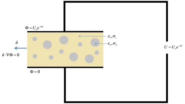
Figure 3. Schematic of the calculation of effective dielectric properties of composites.
So from equations (2) and (3) we obtain
 (5)
(5)
Now using 1, 4 and 5 we can write the following
 (6)
(6)
In case of a sinusoidal applied electric field E of angular frequency

 (7)
(7)
We know
 (8)
(8)
From equation (7) and (8) we get
 (9)
(9)
From equation (9), we can tell that in a heterogeneous material the product of the physical properties (some form of the conductivity and permittivity) and the slope of the potential must be a constant as we cross material boundaries. For the quasi-static case with harmonic input fields, the gradient of that product vanishes. The interacting field is a result of the charge difference at the interface, and unless the conductivity and permittivity of adjacent material phases are identical, there is a disruption of charge transfer at the material boundary which results in internal polarization.
To solve equation (9), we set the potential on the top electrode to be,
 (10)
(10)
And on the bottom electrode,
 (11)
(11)
Boundary conditions on the interfaces are,
 (12)
(12)
 (13)
(13)
where
 is the unit vector normal to the interface surface. To eliminate fringe effects on the side planes, we set
 (14)
(14)
here
 is the unit vector normal to the side plane.
3. Results and Discussion
3.1. Two Phase Model
For this model, an undamaged composite material is considered to be a homogeneous material and the cracks (here as circular inclusions) are considered to be the second phase inside of that homogeneous material system. Permittivity and ohmic conductivity of the host material were taken to be
 and
and
 S/m and for the inclusion permittivity and ohmic conductivity,
 and
and
 S/m, were chosen which are values close to those of the ambient air permittivity and conductivity [7] . Because of the difference in the permittivities and conductivities of the phases, the accumulation of charge at the interphase boundaries causes an undulation of the space distribution of the potential which is shown in the Figure 4 and Figure 5. Figure 4 shows the potential distribution around the inclusion and Figure 5 shows the potential distribution along the horizontal center line. It can be seen that around the boundary of the phases there is a potential nonlinearity (in the figure the nonlinearity is shown inside two ellipses) that is caused by the charge accumulation at the interface between the host material and inclusion. Figure 6 shows that the space charge accumulation is higher, which is caused by the dissimilarity of the material properties around the inclusion boundary in the presence of the applied electric field.
Computer simulations were performed for different volume fractions of the inclusions. Figure 7 shows that the space charge density increases with an increase of the inclusion volume fraction. In the frequency range above 1 Hz the space charge density is constant but below 1 Hz a nonlinear increase is observed in the space charge density around the inclusion interface as shown in Figure 8.
Figure 9 shows the change of the real and imaginary parts of the global permittivities with the increase of volume fraction of the inclusion as a function of frequency. At a high frequency the period of potential oscillations is not sufficient for charge accumulation but at low frequency the charge has enough time to accumulate around the interface which leads to interfacial polarization (Maxwell-Wagner-Sillar polarization); that is why there is an increase in the real part of the permittivity (shown in Figure 10) and dielectric loss at the lower frequencies.
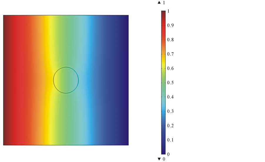
Figure 4. Potential distributions around the inclusion.

Figure 5. Potential distributions along the line.

Figure 6. Space charge densities along the line.
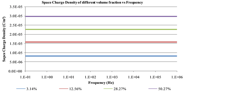
Figure 7. Space charge densities around the inclusion interface of different volume fraction in different frequency.
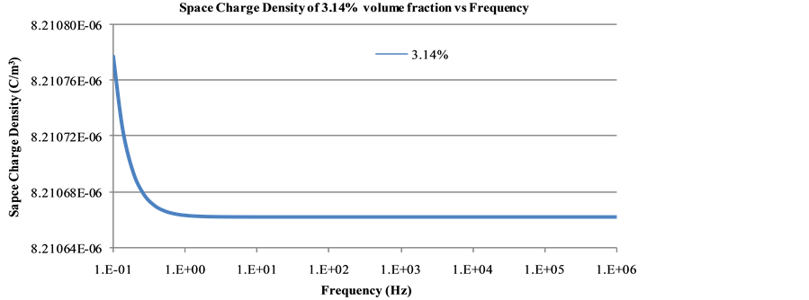
Figure 8. Space charge density change of 3.14% volume fraction of inclusion with frequency.
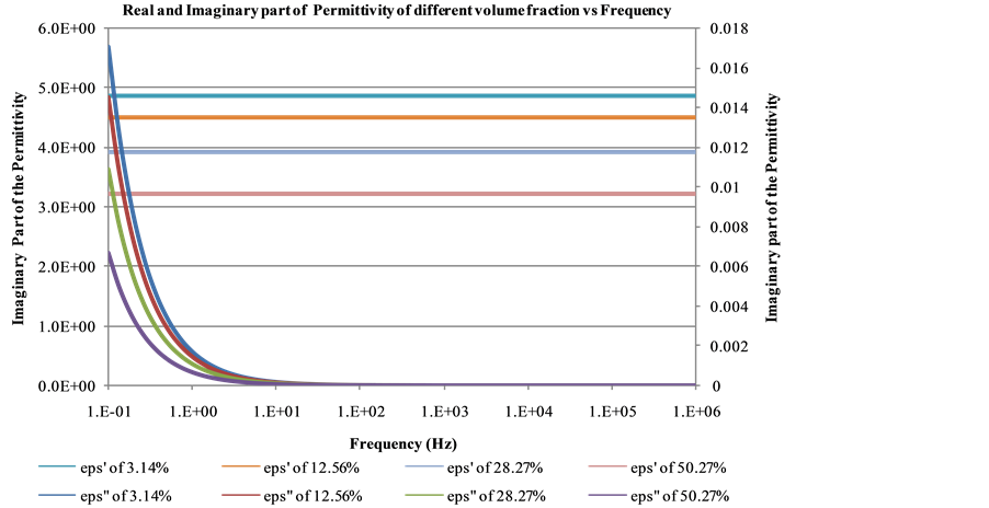
Figure 9. Real and imaginary part of the permittivity with different volume fraction of the inclusion.
For different volume fractions of inclusion, the real part of the permittivity was calculated from the computer simulation for a frequency of 10 Hz. Figure 11 is the comparison of real part of the permittivity change with increasing volume fraction of the inclusion phase. The relation between the real part of the permittivity and volume fraction is almost linear, but when the real part of the permittivity is plotted with surface area fraction (surface area fraction is the ratio of inclusion surface to the material surface) of the inclusion there is clearly a nonlinear relationship predicted. For low volume fractions the effect of surface area fraction of the inclusion is more dominant than the volume fraction, but for the higher volume fractions it is opposite.
Figure 12 illustrates the comparison between computer simulation results with increasing inclusion volume/ surface-area fraction and experimental results. Figure 12(a) and Figure 12(b) show slight increases in the real part of the impedance for low volume/surface-area fractions. Figure 12(c) shows the experimental results for the real part of the impedance change with the strain. The real part of the impedance increases below the low strain (below 5%) for the off axis sample where matrix microcracking is dominant and distributed throughout the material system.
3.2. Three Phase Model
Composite materials are filled with various additive materials to achieve the desired mechanical, thermal and electrical properties. Typical filler materials used for the present modeling are carbon or glass fibers. The use of these fibers as filler materials introduces a water sensitive component into the polymer composites. Glass fibers are well known for their water affinity on their surfaces. Currently, epoxies are widely used matrix materials in
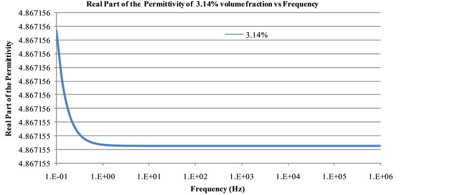
Figure 10. Real part of the permittivity of the material with 3.14% volume fraction of inclusion.

Figure 11. Eps' comparison with volume fraction and surfacearea fraction of the inclusion.
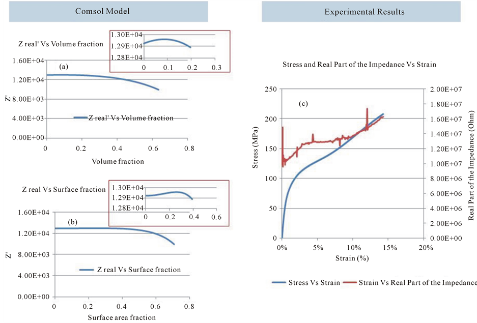
Figure 12. Comparison of ComsolTM simulation result and experimental results.
composite industries, which also have the potential of being sensitive to moist conditions or humid environments. Soles and Yee [8] found that a network of nanopores that is inherent in the epoxy structure helps free water to traverse the epoxy; they found the average size of nanopore diameters to vary from 5 to 6.1 Å and account for 3% - 7% of the total volume of the epoxy material. The approximate diameter of a kinetic water molecule is just 3.0 Å, so via the nanopores network the moisture can easily traverse into the epoxy. They also found that the volume fraction of nanopores does not affect the diffusion coefficient of water and argued that polar groups coincident with the nanopores are the rate-limiting factor in the diffusion process, which could explain why the diffusion coefficient is essentially independent of the nanopore content. In their Figure 13 they explain how the water transport happens in epoxy networks.
There are many theories about the state of water molecules in polymers. Adamson [9] suggested that moisture can transfer in epoxy resins in the form of either liquid or vapor. It is proposed by Tencer [10] that it is also possible that vapor water molecules undergo a phase transformation and condense to the liquid phase. This condensed moisture was stated to be either in the form of discrete droplets on the surface or in the form of a uniform monolayer [11] .
Water has a higher dielectric permittivity and conductivity than the glass fiber and matrix, so it has strong effects on the dielectric properties, i.e. relative permittivity and dielectric loss, of the material system. In the literature it is well established that water absorption increases the dielectric constant of the dielectric material [12] -[16] . This dielectric loss is observed in the low frequency range. Water diffuses through the interface and also weakens the interfacial strength of filler and matrix.
When composite materials go through degradation processes, microcracks typically form and these micro- cracks can also be filled with moist air, and condensed or adsorbed water layers can form on the surface of those defects. In our two phase model we saw an interfacial polarization (Maxwell-Wagner-Sillars polarization) that is present in the low frequency region of the frequency spectra. If a water layer is present on the surface of the defect it will become electrically conductive. Since the host material and defect have low electrical conductivity and permittivity is not significantly high, this will give rise to interfacial polarization.
Figure 14 illustrates the tri-layer computational model used for the study where yellow, gray and blue parts represent respectively the host material, defect, and a conductive layer. The permittivity and ohmic conductivity of the host material were taken to be
 and
and
 S/m and for the inclusion the permittivity and ohmic conductivity had values of
 and
and
 S/m. For the conductive layer a different permittivity
 and conductivity
 (higher than host and defect properties) was used to see the effect on the effective dielectric properties of the material system.
Figure 15 shows the potential distributions around the inclusion of the tri-layer model which is different than the potential difference shown in Figure 4 for the two phase inclusion model. Because of the conductive layer around the inclusion there is a large undulation of the space distribution of the electric potential.

Figure 13. A plausible picture of moisture diffusion through the nanopores of an amine- containing epoxy (Figure from reference [7] ).

Figure 14. Tri-layer model.

Figure 15. Potential distributions around the inclusion with a conductive layer.
For the tri-layer model, the total volume fraction is the sum of the volume fraction of the defect and the volume fraction of the conductive layer. For all of the cases of tri-layer modelling, the conductive layer thickness was specified as 0.5 micro meter. We observed that for two phase models, the real part of the permittivity was almost linear but in Figure 16 we can see that for the three phase case there is an increase in real part of the permittivity for lower volume fractions and then a decreasing trend. As there is a conductive layer in between the defect and the host matrix, the interfacial polarization plays a vital role for this type of behavior. The subsequent decrease of the real part of the permittivity for higher volume fractions is caused by the dominance of the volume of the defects which is higher than the interfacial polarization contributed by the conductive layer.
It is also clear from Figure 17 that for the same conductivity and permittivity values of the conductive layer, for low frequency the real part of the permittivity of the material system is higher than the value for higher frequency.
Figure 18 shows the dependence of dielectric constant on the conductivity of the conductive layer. The real part of the permittivity at different volume fractions for the same permittivity and frequency behave differently for different surface layer conductivities.
As shown in Figure 19, for the same volume fraction of the inclusion but variable frequency of the input field, there is a step-like increase of the real part of the permittivity over a narrow frequency range, and the dielectric loss also has the peak in that region, where the Maxell-Wagner-Sillars polarization dominates.
Figure 20 shows the relation of the real part of the permittivity with the frequency for all volume fractions of the inclusion. That simulation was also done for just the matrix material (this is the host material, as we considered it homogeneous). Since there were no other phases presents for that case, there was no chance of charge accumulation and there is no predicted change of the dielectric constant for the matrix-only case. We can see for higher volume fractions the dielectric relaxation strength (difference between the real parts of the permittivity at low frequency and high frequency) also increases. At higher frequency the real part of the permittivity drops as a function of volume fraction because charge accumulation does not occur at the interface at those frequencies.
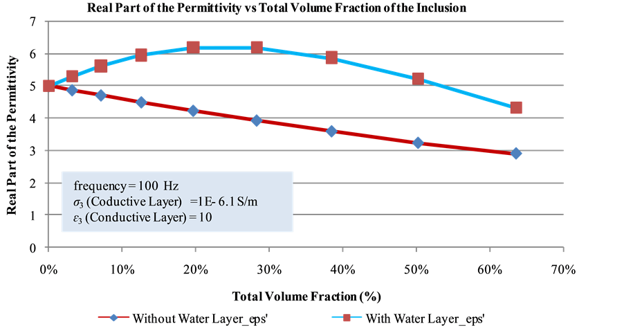
Figure 16. Variation of real part of the permittivity with increasing volume fraction. For the tri-layer model, total volumefraction is the sum of the volume fraction of defect.
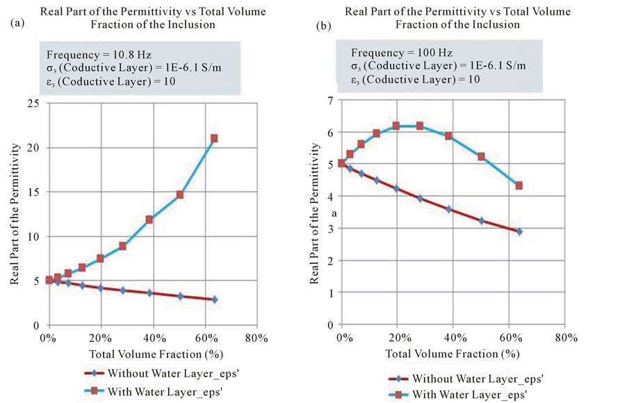
Figure 17. Frequency dependency of the real part of permittivity for different volume fraction.
Dielectric loss (the imaginary part of the permittivity) also varies with volume fraction and it is illustrated in Figure 21. For high volume fraction dielectrics, the loss changes somewhat and the peak of the loss also increases.
The corresponding Cole-Cole plot, Figure 22, also shows the shift in relaxation for different volume fractions.


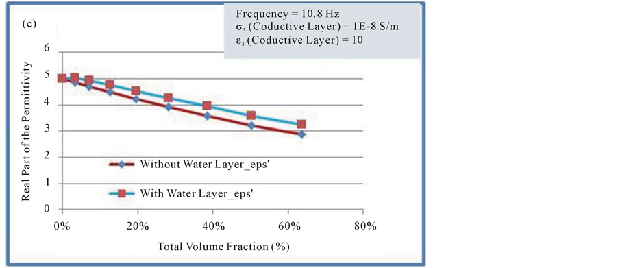
Figure 18. Dielectric properties dependence on the conductivity.

Figure 19. Real and imaginary part of the permittivity Vs frequency for 3.14% total volume fraction of the inclusion.

Figure 20. Real part of the permittivity in frequency spectra of all volume fractions.
3.3. Distributed Damage Model
A distributed damage model was created to see the effect of the distribution of the damage. A dielectric study was performed for a certain volume fraction of inclusion, and then that inclusion was divided into 10 inclusions while keeping the total volume fraction the same.
Figures 23-26 show the change of dielectric properties of a single damage volume and distributed damage volumes with the same amount of volume fraction without any conductive layer around the defects. The dielectric loss increased for the distributed damage because of the presence of more interfacial polarization.

Figure 21. Imaginary part of the permittivity in frequency spectra of all volume fractions.

Figure 22. Cole-Cole plot of different volume fraction.
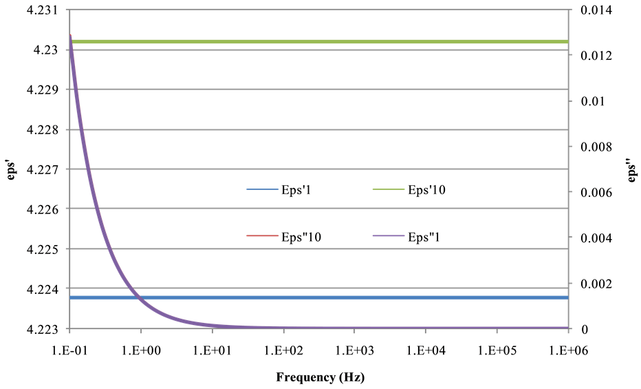
Figure 23. Dielectric Properties without conductive layer for same volume fraction but different number of inclusion.

Figure 24. Real Part of the permittivity for different number of inclusion but same volume fraction.
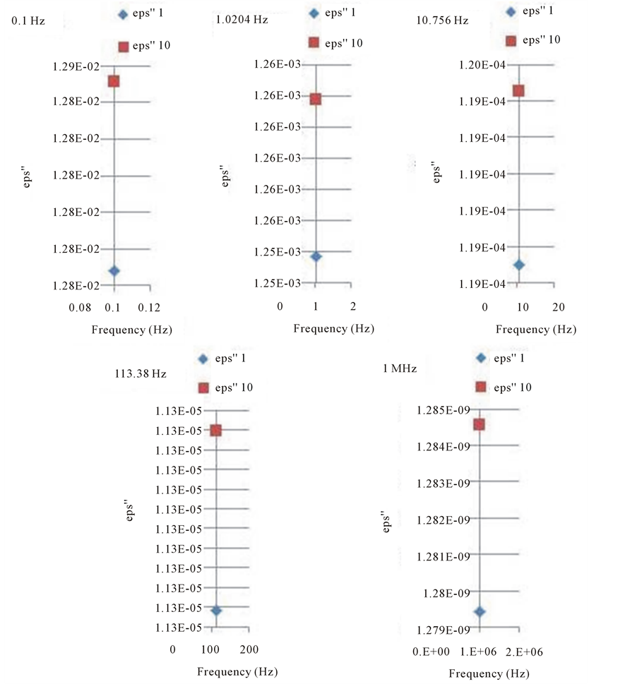
Figure 25. Dielectric losses at different frequency for different number of inclusion but same volume fraction without any conductive layer.
Figures 27-29 show the change of dielectric properties of a single damage phase and distributed damage with the same amount of volume fraction with a conductive layer around the defect. The dielectric loss increased for the distributed damage because of more interfacial polarization and it is more evident than the prior case because the conductive layer around the defect leads to increased interfacial polarization.
The difference between the static permittivity and the limiting high frequency dielectric permittivity is called the Dielectric relaxation strength (DRS),
 , as given in Equation (15).
 (15)
(15)
where,
 is the static permittivity and
 is the limiting high frequency dielectric constant. To calculate DRS from the experimental data we subtract the value of real part of the permittivity at 1 MHz from the value of real part of the permittivity at 0.1 Hz.

Figure 26. Cole-Cole plot of different number of inclusion without conductive layer.
Figure 30(a) shows the increase of DRS with the increase of damage state defects which is in agreement with what we saw in the computational data (Figure 20 and Figure 27). Figure 30(b) shows the increase in dielectric loss with the increase of damage, and this loss increased more in the lower frequency region when the defects had conductive solution layers on their surface, which in also in agreement with the computational model (Figure 21 and Figure 28).
4. Conclusions
In this paper, we have demonstrated a computational model to predict global dielectric property changes caused by increasing defects inside of a materials system. We show that the dielectric character of the defects, their volume, and the morphology of the defect surfaces play an important role in the overall dielectric properties of the materials system during degradation. The data presented here also demonstrate the possibility of using dielectric properties to model and interpret the progressive damage of heterogonous materials systems.

Figure 27. Real part of the Permittivity of different number inclusion but same volume fraction with conductive layer.

Figure 28. Imaginary part of the Permittivity of different number inclusion but same volume fraction with conductive layer.

Figure 29. Cole-Cole plot of different number of inclusion with conductive layer.

Figure 30. Experimental results of dielectric properties change of damaged composite materials.
In general, we have shown that the dielectric properties of heterogeneous systems are influenced by various physical factors: electrical and structural interactions between particles, heterogeneity of morphological and electrical properties of the constituent phases, frequency dependence of electrical phase parameters, intra-parti- cle structure, particle shape, size, orientation and, volume and surface fraction of the constituent phases. This dependence complicates the determination of the electrical parameters of heterogeneous materials from the observed global dielectric relaxation spectra, but also presents us with an opportunity to recover important information not only about the electrical and structural properties of constituents but also about the interactions between constituents, including the parent materials and damage phases. Further theoretical and experimental investigation is required to fully understand the changes in dielectric spectra associated with many of the specific damage accumulation events and local details in heterogeneous material systems.
From the results presented in this paper, it can be concluded that analysis of the dielectric data gives us information about the type of material state changes throughout the mechanical life of a composite material. It should be emphasized that these changes in the dielectric properties are distinct and measurable changes in material state, and that they are caused by a non-conservative, non-equilibrium material response to the applied fields. Opportunities for further understanding include the identification of the material and physical limitations of this method of characterization, e.g., specimen size, material property ranges, and specimen shapes that are most and least suited to the approach. A robust study of the interpretation of dielectric data associated with specific damage modes and details is also needed.
Cite this paper
RasselRaihan,FazleRabbi,VamseeVadlamudi,KennethReifsnider, (2015) Composite Materials Damage Modeling Based on Dielectric Properties. Materials Sciences and Applications,06,1033-1053. doi: 10.4236/msa.2015.611103
References
- 1. Reifsnider, K.L. and Case, S.W. (2002) Damage Tolerance and Durability of Material Systems. John Wiley and Sons, New York.
- 2. Raihan, R., Adkins, J.M., Baker, J., Rabbi, F. and Reifsnider, K. (2014) Relationship of Dielectric Property Change to Composite Material State Degradation. Composites Science and Technology, 105, 160-165.
http://dx.doi.org/10.1016/j.compscitech.2014.09.017 - 3. Raihan, R., Reifsnider, K., Cacuci, D. and Liu, Q. (2015) Dielectric Signatures and Interpretive Analysis for Changes of State in Composite Materials. ZAMM-Journal of Applied Mathematics and Mechanics/Zeitschrift für Angewandte Mathematik und Mechanik.
http://dx.doi.org/10.1002/zamm.201400226 - 4. Tuncer, E., Serdyuk, Y.V. and Gubanski, S.M. (2001) Dielectric Mixtures—Electrical Properties and Modeling.
- 5. Brosseau, C., Beroual, A. and Boudida, A. (2000) How Do Shape Anisotropy and Spatial Orientation of the Constituents Affect the Permittivity of Dielectrich Eterostructures? Journal of Applied Physics, 88, 7278-7288.
http://dx.doi.org/10.1063/1.1321779 - 6. Baker, J., Adkins, J.M., Rabbi, F., Liu, Q., Reifsnider, K. and Raihan, R. (2014) Meso-Design of Heterogeneous Dielectric Material Systems: Structure Property Relationships. Journal of Advanced Dielectrics, 4, 1450008.
http://dx.doi.org/10.1142/S2010135X14500088 - 7. Pawar, S.D., Murugavel, P. and Lal, D.M. (2009) Effect of Relative Humidity and Sea Level Pressure on Electrical Conductivity of Air over Indian Ocean. Journal of Geophysical Research: Atmospheres, 114(D2).
- 8. Soles, C. and Yee, A. (2000) A Discussion of the Molecular Mechanisms of Moisture Transport in Epoxy Resins. Journal of Polymer Science, Part B: Polymer Physics, 38, 792-802.
http://dx.doi.org/10.1002/(SICI)1099-0488(20000301)38:5<792::AID-POLB16>3.0.CO;2-H - 9. Adamson, M.J. (1980) Thermal Expansion and Swelling of Cured Epoxy Resin Used in Graphite/Epoxy Composite Materials. Journal of Material Science, 15, 1736-1745.
http://dx.doi.org/10.1007/bf00550593 - 10. Tencer, M. (1994) Moisture Ingress into Nonhermetic Enclosures and Packages—A Quasisteady State Model for Diffusion and Attenuation of Ambient Humidity Variations. IEEE 44th Electronic Components Technology Conference, Washington DC.
- 11. Shirangi, M.H. and Michel, B. (2010) Mechanism of Moisture Diffusion, Hygroscopic Swelling, and Adhesion Degradation in Epoxy Molding Compounds. Moisture Sensitivity of Plastic Packages of IC Devices, Springer, 29-69.
http://dx.doi.org/10.1007/978-1-4419-5719-1_2 - 12. Banhegyi, G. and Karasz, F.E. (1986) The Effect of Adsorbed Water on the Dielectric Properties of CaCO3 Filled Polyethylene Composites. Journal of Polymer Science Part B: Polymer Physics, 24, 209-228.
http://dx.doi.org/10.1002/polb.1986.090240201 - 13. Banhegyi, G., Hedvig, P. and Karasz, F.E. (1988) DC Dielectric Study of Polyethylene/CaCO3 Composites. Colloid and Polymer Science, 266, 701-715.
http://dx.doi.org/10.1007/BF01410279 - 14. Cotinaud, M., Bonniau, P. and Bunsell, A.R. (1982) The Effect of Water Absorption on the Electrical Properties of Glass-Fibre Reinforced Epoxy Composites. Journal of Materials Science, 17, 867-877.
http://dx.doi.org/10.1007/bf00540386 - 15. Reid, J.D., Lawrence, W.H. and Buck, R.P. (1986) Dielectric Properties of an Epoxy Resin and Its Composite I. Moisture Effects on Dipole Relaxation. Journal of Applied Polymer Science, 31, 1771-1784.
http://dx.doi.org/10.1002/app.1986.070310622 - 16. Paquin, L., St-Onge, H. and Wertheimer, M.R. (1982) The Complex Permittivity of Polyethylene/Mica Composites. IEEE Transactions on Electrical Insulation, 5, 399-404.
http://dx.doi.org/10.1109/TEI.1982.298482
NOTES

*Corresponding author.