ABSTRACT

In this paper, a nonautonomous eco-epidemiological model with disease in the predator is formulated and analyzed, in which saturated predation rate is taken into consideration. Under quite weak assumptions, sufficient conditions for the permanence and extinction of the disease are obtained. Moreover, by constructing a Liapunov function, the global attractivity of the model is discussed. Finally, numerical simulations verified these results.

Keywords:

Nonautonomous, Eco-Epidemiological Model, Permanence, Extinction, Global Attractivity

1. Introduction

In the nature world, diseases for each species are inevitable. So it has practical ecological significance to consider the effects of disease in predator-prey model. Over the past decade, great attention has been paid to modelling and analyzing eco-epidemiological systems (see [1] - [25] ). Most of these works studied predator-prey models with disease in the prey (see [1] - [21] [25] ). Recently different eco- epidemiological predator-prey models with disease in predator have been investigated (see [22] [23] [24] ). In [21] , Xiao et al. considered the following autonomous predator-prey model with disease in predator:

$\{\begin{array}{l}\frac{\text{d}x}{\text{d}t}=x\left[r_1-ax-b_1{y}_1-b_2{y}_2\right],\hfill \\ \frac{\text{d}{y}_1}{\text{d}t}=y_1\left[r_2+cx-d_1\left(y_1+y_2\right)-\beta y_2\right],\hfill \\ \frac{\text{d}{y}_2}{\text{d}t}=y_2\left[\beta y_1-d_2\left(y_1+y_2\right)\right],\hfill \end{array}$ (1.1)

where $x\left(t\right)$ denotes the number of wild plant species at time t; $y_1\left(t\right)$ and $y_2\left(t\right)$ denote the number of susceptible pest and infected pest at time t, respectively. Boundedness of solutions, equilibria, permanence and global stability is analyzed. Numerical simulations show that the system exhibits complex dynamics including quasiperiodic solution, chaotic attractors when the transmission rate varies periodically.

The models, which were proposed in the literatures [1] - [21] , are autonomous systems. However, non-autonomous phenomenon is dominating in real systems. It comes from various sources, such as the variation of transmission rate, migration rate, the predation rate and fluctuations in death and birth rates, etc. Nonautonomous eco-epidemiological model is more realistic than autonomous model. Several nonautonomous eco-epidemiological models have been studied in [25] [26] [27] [28] [29] . In addition, different infection rates and predation rates have been suggested by authors: the term of the infection rate is bilinear $\beta SI$ in [1] - [12] [14] [15] [16] [17] [18] [20] [21] ; in [13] , the infection rate is nonlinear $b{I}^{2}S$ ; in [19] , the infection rate is saturated $\beta SI/\left(1+\alpha I\right)$ ; the term of the predation rate is linear pIY in [3] [5] [10] [11] [13] [15] [16] [17] [20] [21] ; but in [1] [2] [6] [7] [8] [9] [12] [14] [18] [19] , the predation rate is saturated $mYI/\left(A+I\right)$ .

Motivated by these factors, we modify a predator-prey model with disease in predator by introducing standard infection rate $\sigma \left(t\right)S\left(t\right)I\left(t\right)/\left(S\left(t\right)+I\left(t\right)\right)$ and saturated predation rate $c\left(t\right)X\left(t\right)S\left(t\right)/\left(h\left(t\right)+X\left(t\right)\right)$ , more in line with the actual situation, where prey population denoted by X and predator population denoted by $Y\left(t\right)=S\left(t\right)+I\left(t\right)$ , in which S and I stand for the susceptible and infectious predator, respectively. Then we propose the following nonautonomous eco-epidemiological model:

$\{\begin{array}{l}\frac{\text{d}X\left(t\right)}{\text{d}t}=A\left(t\right)-d\left(t\right)X\left(t\right)-c\left(t\right)\frac{X\left(t\right)}{h\left(t\right)+X\left(t\right)}\left(S\left(t\right)+{\rho }_{0}I\left(t\right)\right),\hfill \\ \begin{array}{l}\frac{\text{d}S\left(t\right)}{\text{d}t}=S\left(t\right)\left(r\left(t\right)-b\left(t\right)\left(S\left(t\right)+I\left(t\right)\right)\right)+e\left(t\right)c\left(t\right)\frac{X\left(t\right)S\left(t\right)}{h\left(t\right)+X\left(t\right)}\\ -\sigma \left(t\right)\frac{S\left(t\right)I\left(t\right)}{S\left(t\right)+I\left(t\right)},\end{array}\hfill \\ \begin{array}{l}\frac{\text{d}I\left(t\right)}{\text{d}t}=I\left(t\right)\left(r\left(t\right)-b\left(t\right)\left(S\left(t\right)+I\left(t\right)\right)\right)+{\rho }_{0}e\left(t\right)c\left(t\right)\frac{X\left(t\right)I\left(t\right)}{h\left(t\right)+X\left(t\right)}\\ +\sigma \left(t\right)\frac{S\left(t\right)I\left(t\right)}{S\left(t\right)+I\left(t\right)}-\alpha \left(t\right)I\left(t\right),\end{array}\hfill \end{array}$ (1.2)

where $A\left(t\right)$ is the recruitment rate of prey; $d\left(t\right)$ is the natural death rates of prey; $c\left(t\right)$ is the predation rate of predator; $h\left(t\right)$ is half-saturation rate; constant ${\rho }_0\left(0<{\rho }_0<1\right)$ is predation capacity of infection; $e\left(t\right)$ is the coefficient in conversing prey into new immature predator; $r\left(t\right)$ is the intrinsic recruitment rate of predator; $b\left(t\right)$ is the natural death rates of predator; $\sigma \left(t\right)$ is the contact rate; $\alpha \left(t\right)$ is the disease-related death rate of predator.

The initial conditions are

$X\left(0\right)>0,S\left(0\right)>0,I\left(0\right)\ge 0.$ (1.3)

It is obvious that the set $K=\left\{\left(X,S,I\right)\in R^3|X\ge 0,S\ge 0,I\ge 0\right\}$ is a positively invariant set of system (1.2).

This paper is organized as follows. In the next section, some useful lemmas are proposed. In Section 3, we establish the sufficient conditions for the permanence and extinction of the disease. Also, by constructing a Liapunov function, we obtain the global attractivity of the model. Moreover, as applications of the main results, some corollaries are introduced. Particularly, the periodic model is discussed. In Section 4, our qualitative results for the periodic system are verified by numerical simulation. This paper is ended with a conclusion.

2. Notations, Definitions, and Preliminary Lemmas

In this section, we introduce some notations, definitions and state some lemmas which will be useful in the subsequent sections. Let C denote the space of all bounded continuous functions. Given $f\in C$ , we let

$f^u=\underset{t\to \infty }{{\displaystyle \lim \sup }}f\left(t\right),f^v=\underset{t\to \infty }{{\displaystyle \lim \inf }}f\left(t\right).$

If $f$ is W-periodic, then the average value of $f$ on a time interval $\left[0,W\right]$ can be defined as

$\overline{f}=\frac{1}{W}{\displaystyle {\int }_0^W}f\left(t\right)\text{d}t.$

Definition 2.1. System (1.2) is said to be permanent if there exists a compact region $K_0\subset K$ such that every solution of system (1.2) with initial conditions (1.3) will eventually enter and remain in the region $K_0$ .

Definition 2.2. The disease is said to be extinct if the solution of system (1.2) with initial conditions (1.3) satisfy $\underset{t\to \infty }{\lim }I\left(t\right)=0$ .

Definition 2.3. The system (1.2) is said to be globally attractive if for any two solutions $\left(X_1\left(t\right),S_1\left(t\right),I_1\left(t\right)\right)$ and $\left(X_2\left(t\right),S_2\left(t\right),I_2\left(t\right)\right)$ of system (1.2) satisfy

$\underset{t\to \infty }{\lim }\left|X_1\left(t\right)-X_2\left(t\right)\right|=0,\underset{t\to \infty }{\lim }\left|S_1\left(t\right)-S_2\left(t\right)\right|=0,\underset{t\to \infty }{\lim }\left|I_1\left(t\right)-I_2\left(t\right)\right|=0.$

To prove our main results, first, we give the results on the following nonautonomous Logistic differential equation:

$\frac{\text{d}x\left(t\right)}{\text{d}t}=x\left(t\right)\left(r\left(t\right)-b\left(t\right)x\left(t\right)\right),$ (2.1)

where functions $r\left(t\right)$ and $b\left(t\right)$ are continuous and bounded on $R_{+}=\left[0,+\infty \right)$ .

Lemma 2.1 [26] If there exist positive constants ${\omega }_i>0\left(i=1,2\right)$ such that

$\underset{t\to +\infty }{\lim \inf }{\displaystyle {\int }_t^{t+{\omega }_1}}r\left(\theta \right)\text{d}\theta >0,\underset{t\to +\infty }{\lim \inf }{\displaystyle {\int }_t^{t+{\omega }_2}}b\left(\theta \right)\text{d}\theta >0.$

Then

(a) There exist $m,M>0$ , such that every positive solution of Equation (2.1), $x\left(t\right)$ satisfies

$m<\underset{t\to \infty }{\lim \inf }x\left(t\right)\le \underset{t\to \infty }{\lim \sup }x\left(t\right)<M.$

(b) Each fixed solution $x^{\ast }\left(t\right)$ of Equation (2.1) with initial value $x^{\ast }\left(0\right)>0$ is bounded and globally uniformly attractive on $R_{+}$ .

(c) If $b^v>0$ , then for any solution $x\left(t\right)$ of Equation (2.1) with initial value $x\left(0\right)>0$ , we get

${\left(\frac{r}{b}\right)}^v\le \underset{t\to \infty }{\lim \inf }x\left(t\right)\le \underset{t\to \infty }{\lim \sup }x\left(t\right)\le {\left(\frac{r}{b}\right)}^u.$

(d) When Equation (2.1) is W-periodic, then Equation (2.1) has a unique nonegative W-periodic solution which is globally uniformly attractive.

Second, we consider the following equation:

$\frac{\text{d}x\left(t\right)}{\text{d}t}=x\left(t\right)\left(r\left(t\right)-b\left(t\right)x\left(t\right)+k\left(t\right)\right),$ (2.2)

where functions $r\left(t\right)$ and $b\left(t\right)$ are defined as in Equation (2.1) and $k\left(t\right)$ is continuous and bounded function on $R_{+}$ . Let $x\left(t,t_0,x_0\right)$ is the solution of Equation (2.2) with initial value $x\left(t_0\right)=x_0$ and $x_0\left(t\right)$ is a fixed positively solution of Equation (2.1). Then we get the following lemma.

Lemma 2.2 If there exist positive constants ${\omega }_i>0\left(i=1,2\right)$ such that

$\underset{t\to +\infty }{\lim \inf }{\displaystyle {\int }_t^{t+{\omega }_1}}r\left(\theta \right)\text{d}\theta >0,\underset{t\to +\infty }{\text{liminf}}{\displaystyle {\int }_t^{t+{\omega }_2}}b\left(\theta \right)\text{d}\theta >0.$

Then for any constants ε > 0 and $\tilde{M}>0$ , there exist constants $\delta =\delta \left(\epsilon \right)>0,$ $T=T\left(\epsilon ,\tilde{M}\right)>0$ , such that for any $t_0\in R_{+}$ and $x_0\in \left[{\tilde{M}}^{-1},\tilde{M}\right]$ , when $\left|k\left(t\right)\right|\le \delta$ for all $t\ge t_0$ we get

$\left|x\left(t,t_0,x_0\right)-x_0\left(t\right)\right|<\epsilon \text{forall}t\ge t_0+T,$

Lemma 2.2 can be easily proved and hence we omit it here.

Third, we give the following nonautonomous linear differential equation

$\frac{\text{d}x\left(t\right)}{\text{d}t}=A\left(t\right)-d\left(t\right)x\left(t\right),$ (2.3)

where functions $A\left(t\right)$ and $d\left(t\right)$ are continuous and bounded on $R_{+}$ . Then we get the following lemma.

Lemma 2.3 [27] If there exist positive constants ${\omega }_i>0\left(i=3,4\right)$ such that

$\underset{t\to +\infty }{\lim \inf }{\displaystyle {\int }_t^{t+{\omega }_3}}A\left(\theta \right)\text{d}\theta >0,\underset{t\to +\infty }{\lim \inf }{\displaystyle {\int }_t^{t+{\omega }_4}}d\left(\theta \right)\text{d}\theta >0.$

Then

(a) There exist $m,M>0$ , such that every positive solution of Equation (2.3), $x\left(t\right)$ satisfies

$m<\underset{t\to \infty }{\lim \inf }x\left(t\right)\le \underset{t\to \infty }{\lim \sup }x\left(t\right)<M.$

(b) Each fixed solution $x^{\ast }\left(t\right)$ of Equation (2.3) with initial value $x^{\ast }\left(0\right)>0$ is bounded and globally uniformly attractive on $R_{+}$ .

(c) If $d^v>0$ , then for any solution $x\left(t\right)$ of Equation (2.3) with initial value $x\left(0\right)>0$ , we get

${\left(\frac{A}{d}\right)}^v\le \underset{t\to \infty }{\lim \inf }x\left(t\right)\le \underset{t\to \infty }{\lim \sup }x\left(t\right)\le {\left(\frac{A}{d}\right)}^u.$

(d) When Equation (2.3) is W-periodic, then Equation (2.3) has a unique nonegative W-periodic solution which is globally uniformly attractive.

Finally, we investigate the following equation

$\frac{\text{d}x\left(t\right)}{\text{d}t}=A\left(t\right)-d\left(t\right)x\left(t\right)+k\left(t\right),$ (2.4)

where functions $A\left(t\right)$ and $d\left(t\right)$ are defined as in Equation (2.3) and $k\left(t\right)$ is continuous and bounded function on $R_{+}$ . Let $x\left(t,t_0,x_0\right)$ is the solution of Equation (2.4) with initial value $x\left(t_0\right)=x_0$ and $x_0\left(t\right)$ is a fixed positive solution of Equation (2.3). Then we get the following lemma.

Lemma 2.4 [28] If there exist positive constants ${\omega }_i>0\left(i=3,4\right)$ such that

$\underset{t\to +\infty }{\lim \inf }{\displaystyle {\int }_t^{t+{\omega }_3}}A\left(\theta \right)\text{d}\theta >0,\underset{t\to +\infty }{\lim \inf }{\displaystyle {\int }_t^{t+{\omega }_4}}d\left(\theta \right)\text{d}\theta >0.$

Then for any constants ε > 0 and $\tilde{M}>0$ , there exist constants $\delta =\delta \left(\epsilon \right)>0,$ $T=T\left(\epsilon ,\tilde{M}\right)>0$ , such that for any $t_0\in R_{+}$ and $\left|x_0\right|\le \tilde{M}$ , when $\left|k\left(t\right)\right|\le \delta$ for all $t\ge t_0$ we get

$\left|x\left(t,t_0,x_0\right)-x_0\left(t\right)\right|<\epsilon \text{forall}t\ge t_0+T\mathrm{,}$

3. Main Results

In this section, we will study the permanence and extinction of infected predator, and then, demonstrate the global attractivity of system (1.2).

First, as a preliminary, we make the following assumptions:

(B1) Functions $A\left(t\right),d\left(t\right),c\left(t\right),h\left(t\right),b\left(t\right),e\left(t\right),\sigma \left(t\right),\alpha \left(t\right)$ are all nonnegative, continuous and bounded on $R_{+}=\left[0,+\infty \right)$ ; and $r\left(t\right)$ is continuous and bounded on $R_{+}=\left[0,+\infty \right)$ ;

(B2) There exist positive constant ${\omega }_i>0\left(i=1,2,3,4\right)$ such that

$\begin{array}{l}\underset{t\to +\infty }{\lim \inf }{\displaystyle {\int }_t^{t+{\omega }_1}}r\left(\theta \right)\text{d}\theta >0,\underset{t\to +\infty }{\lim \inf }{\displaystyle {\int }_t^{t+{\omega }_2}}b\left(\theta \right)\text{d}\theta >0,\hfill \\ \underset{t\to +\infty }{\lim \inf }{\displaystyle {\int }_t^{t+{\omega }_3}}A\left(\theta \right)\text{d}\theta >0,\underset{t\to +\infty }{\lim \inf }{\displaystyle {\int }_t^{t+{\omega }_4}}d\left(\theta \right)\text{d}\theta >0,\hfill \end{array}$

Next, we will discuss the ultimate boundness and the permanence of prey and predator of system (1.2).

Theorem 3.1 Suppose that assumptions (B1) and (B2) hold, if there exists a constant ${\omega }_5>0$ , such that

$\left(B3\right)\underset{t\to +\infty }{\lim \inf }{\displaystyle {\int }_t^{t+{\omega }_5}}\left(r\left(\theta \right)-\alpha \left(\theta \right)+{\rho }_{0}e\left(\theta \right)c\left(\theta \right)\frac{m_1}{h\left(\theta \right)+m_1}\right)\text{d}\theta \mathrm{<mo>\; >\; </mo>\; 0,}$

hold, where $m_1={\left(\frac{Ah}{dh+c{M}_2}\right)}^v,M_2={\left(\frac{rh+r{M}_1+ec{M}_1}{bh+b{M}_1}\right)}^u,M_1={\left(\frac{A}{d}\right)}^u$ . Then the

prey population $X\left(t\right)$ and the predator population $\begin{array}{r}\hfill Y\left(t\right)=S\left(t\right)+I\left(t\right)\end{array}$ of system (1.2) are permanent.

Proof. Let $\left(X\left(t\right),S\left(t\right),I\left(t\right)\right)$ be any positive solution of system (1.2) with initial conditions (1.3). From the first equation of (1.2), we can obtain that for all $t\ge 0$

$\begin{array}{c}\frac{\text{d}X\left(t\right)}{\text{d}t}=A\left(t\right)-d\left(t\right)X\left(t\right)-c\left(t\right)\frac{X(t)}{h\left(t\right)+X\left(t\right)}\left(S\left(t\right)+{\rho }_{0}I\left(t\right)\right)\\ \le A\left(t\right)-d\left(t\right)X\left(t\right).\end{array}$ (3.1)

Based on the assumption (B2), the conclusion (a) of Lemma 2.3 and the com- parison theorem, there exist constant $M_1,T_1>0$ , such that

$X\left(t\right)\le M_1,\text{for}t\ge T_1.$ (3.2)

If $d^v>0$ , according to the conclusion (c) of lemma 2.3, then we get

$M_1={\left(\frac{A}{d}\right)}^u$ .

From the second and third equations of (1.2) and (3.2), we have obtain that for all $t\ge T_1$

#Math_125# (3.3)

Based on the assumption (B2), we have

$\underset{t\to +\infty }{\lim \inf }{\displaystyle {\int }_t^{t+{\omega }_1}}\left(r\left(\theta \right)+e\left(\theta \right)c\left(\theta \right)\frac{M_1}{h\left(\theta \right)+M_1}\right)\text{d}\theta >\mathrm{0,}$

According to the conclusion (a) of Lemma 2.1 and the comparison theorem, there exist constant $M_2$ and $T_2\left(\ge T_1\right)$ such that

$S\left(t\right)+I\left(t\right)\le M_2,\text{for}t\ge T_2.$ (3.4)

If $b^v>0$ , according to the conclusion (c) of Lemma 2.1, then we get

$M_2={\left(\frac{rh+r{M}_1+ec{M}_1}{bh+b{M}_1}\right)}^u$ .

Consequently, any solutions $\left(X\left(t\right),S\left(t\right),I\left(t\right)\right)$ of system (1.2) with initial conditions (1.3) are ultimately bounded.

Furthermore, from the first equation of system (1.2) and (3.4), we can obtain that for all $t\ge T_2$

$\begin{array}{c}\frac{\text{d}X\left(t\right)}{\text{d}t}=A\left(t\right)-d\left(t\right)X\left(t\right)-c\left(t\right)\frac{X\left(t\right)}{h\left(t\right)+X\left(t\right)}\left(S\left(t\right)+{\rho }_{0}I\left(t\right)\right)\\ \ge A\left(t\right)-\left(d\left(t\right)+\frac{c\left(t\right)}{h\left(t\right)}{M}_2\right)X\left(t\right).\end{array}$ (3.5)

According to Lemma 2.3 (a) and the comparison theorem, there are constant $m_1,T_3\left(\ge T_2\right)$ , such that

$X\left(t\right)\ge m_1,\text{for}t\ge T_3.$ (3.6)

If $d^v>0$ , according to the conclusion (c) of lemma 2.3, then we get $m_1={\left(\frac{Ah}{dh+c{M}_2}\right)}^v$ .

Moreover, it follows from the second and third equations of system (1.2) and (3.6) that for $t\ge T_3$

$\begin{array}{l}\frac{\text{d}\left(S\left(t\right)+I\left(t\right)\right)}{\text{d}t}=\left(S\left(t\right)+I\left(t\right)\right)\left(r\left(t\right)-b\left(t\right)\left(S\left(t\right)+I\left(t\right)\right)\right)\\ +e\left(t\right)c\left(t\right)\frac{X\left(t\right)}{h\left(t\right)+X\left(t\right)}\left(S\left(t\right)+{\rho }_{0}I\left(t\right)\right)-\alpha \left(t\right)I\left(t\right)\\ \ge \left(S\left(t\right)+I\left(t\right)\right)\left(r\left(t\right)-\alpha \left(t\right)+{\rho }_{0}e\left(t\right)c\left(t\right)\frac{m_1}{h\left(t\right)+m_1}-b\left(t\right)\left(S\left(t\right)+I\left(t\right)\right)\right)\mathrm{.}\end{array}$ (3.7)

Based on the assumption (B3), the comparison theorem and conclusion (a) of Lemma 2.1, there exist constant $m_2,T_4\left(\ge T_3\right)$ such that

$S\left(t\right)+I\left(t\right)\ge m_2,\text{for}t\ge T_4.$ (3.8)

If $b^v>0$ , according to the conclusion (c) of Lemma 2.1, then we get

$m_2={\left(\frac{rh+r{m}_1-\alpha h-\alpha m_1+{\rho }_{0}ec{m}_1}{bh+b{m}_1}\right)}^v$

Therefore, from (3.2), (3.4), (3.6) and (3.8), we can obtain that

$m_1\le \underset{t\to +\infty }{\lim \inf }X\left(t\right)\le \underset{t\to +\infty }{\lim \sup }X\left(t\right)\le M_1,$

and

$m_2\le \underset{t\to +\infty }{\lim \inf }\left(S\left(t\right)+I\left(t\right)\right)\le \underset{t\to +\infty }{\lim \sup }\left(S\left(t\right)+I\left(t\right)\right)\le M_2.$

This completes the proof of Theorem 3.1.

Remark 3.1. Suppose that assumptions (B1), (B2), (B3) hold, and $d^v>0$ ; $b^v>0$ , then we can choose the constants given in the above theorem as following:

$M_1={\left(\frac{A}{d}\right)}^u,M_2={\left(\frac{rh+r{M}_1+ec{M}_1}{bh+b{M}_1}\right)}^u,$

and

$m_1={\left(\frac{Ah}{dh+c{M}_2}\right)}^v,m_2={\left(\frac{rh+r{m}_1-\alpha h-\alpha m_1+{\rho }_{0}ec{m}_1}{bh+b{m}_1}\right)}^v,M_0=m_2^{-1}+M_2.$

Let $x_0\left(t\right)$ be a fixed solution of the nonautonomous linear system

$\frac{\text{d}X\left(t\right)}{\text{d}t}=A\left(t\right)-d\left(t\right)X\left(t\right).$ (3.9)

Particularly, if $d^v>0$ , according to conclusion (c) of Lemma 2.3, we get

${\left(\frac{A}{d}\right)}^v\le \underset{t\to \infty }{\lim \inf }{x}_0\left(t\right)\le \underset{t\to \infty }{\lim \sup }{x}_0\left(t\right)\le {\left(\frac{A}{d}\right)}^u.$

Let $y_0\left(t\right)$ be a fixed solution of the nonautonomous logistic system

$\frac{\text{d}Y\left(t\right)}{\text{d}t}=Y\left(t\right)\left(r\left(t\right)+e\left(t\right)c\left(t\right)\frac{M_2}{h\left(t\right)+M_2}-b\left(t\right)Y\left(t\right)\right).$ (3.10)

If $b^v>0$ , according to conclusion (c) of Lemma 2.1, we get

${\left(\frac{rh+r{M}_2+ec{M}_2}{bh+b{M}_2}\right)}^v\le \underset{t\to \infty }{\lim \inf }{y}_0\left(t\right)\le \underset{t\to \infty }{\lim \sup }{y}_0\left(t\right)\le {\left(\frac{rh+r{M}_2+ec{M}_2}{bh+b{M}_2}\right)}^u.$

Let $y_1\left(t\right)$ be a fixed solution of the nonautonomous logistic system

$\frac{\text{d}Y\left(t\right)}{\text{d}t}=Y\left(t\right)\left(r\left(t\right)-\alpha \left(t\right)+{\rho }_{0}e\left(t\right)c\left(t\right)\frac{m_1}{h\left(t\right)+m_1}-b\left(t\right)Y\left(t\right)\right).$ (3.11)

If $b^v>0$ , according to conclusion (c) of Lemma 2.1, we get

$\begin{array}{c}{\left(\frac{rh+r{m}_1-\alpha h-\alpha m_1+ec{m}_1}{bh+b{m}_1}\right)}^v\le \underset{t\to \infty }{\lim \inf }{y}_0\left(t\right)\\ \le \underset{t\to \infty }{\lim \sup }{y}_0\left(t\right)\\ \le {\left(\frac{rh+r{m}_1-\alpha h-\alpha m_1+ec{m}_1}{bh+b{m}_1}\right)}^u\mathrm{.}\end{array}$

Let $x_1\left(t\right)$ be a fixed solution of the nonautonomous linear system

$\frac{\text{d}X\left(t\right)}{\text{d}t}=A\left(t\right)-\left(d\left(t\right)+\frac{c\left(t\right)}{h\left(t\right)}{M}_2\right)X\left(t\right).$ (3.12)

If ${\left(\frac{dh+c{M}_2}{h}\right)}^v>0$ , according to conclusion (c) of Lemma 2.3, we get

${\left(\frac{Ah}{dh+c{M}_2}\right)}^v\le \underset{t\to \infty }{\lim \inf }{x}_1\left(t\right)\le \underset{t\to \infty }{\lim \sup }{x}_1\left(t\right)\le {\left(\frac{Ah}{dh+c{M}_2}\right)}^u.$

Let $s_0\left(t\right)$ be a fixed solution of the nonautonomous logistic system

$\frac{\text{d}S\left(t\right)}{\text{d}t}=S\left(t\right)\left(r\left(t\right)-b\left(t\right)S\left(t\right)\right).$ (3.13)

If $b^v>0$ , according to conclusion (c) of Lemma 2.1, we get

${\left(\frac{r}{b}\right)}^v\le \underset{t\to \infty }{\lim \inf }{s}_0\left(t\right)\le \underset{t\to \infty }{\lim \sup }{s}_0\left(t\right)\le {\left(\frac{r}{b}\right)}^u.$

Then we can obtain the following results.

Theorem 3.2 Suppose that assumptions (B1), (B2), (B3) hold. If there exists a constant ${\omega }_6>0$ , such that

$\begin{array}{r}\hfill \begin{array}{l}\underset{t\to +\infty }{\lim \inf }{\displaystyle {\int }_t^{t+{\omega }_6}}(r\left(\theta \right)-b\left(\theta \right)y_0\left(\theta \right)+\sigma \left(\theta \right)\frac{s_0\left(\theta \right)}{y_0\left(\theta \right)}\\ +{\rho }_{0}e\left(\theta \right)c\left(\theta \right)\frac{x_1\left(\theta \right)}{h\left(\theta \right)+x_1\left(\theta \right)}-\alpha \left(\theta \right))\text{d}\theta >0,\end{array}\end{array}$ (3.14)

then the infective predator of (1.2) $I\left(t\right)$ is permanent.

Proof. Let $\left(X\left(t\right),S\left(t\right),I\left(t\right)\right)$ be any positive solution of system (1.2). From (3.14), we can choose sufficiently small ${\epsilon }_1>0,{\epsilon }_2>0$ , then there exists $T_0>0$ such that for $t>T_0$ ,

$\begin{array}{r}\hfill \begin{array}{l}{\displaystyle {\int }_t^{t+{\omega }_6}}(r\left(\theta \right)-b\left(\theta \right)\left(y_0\left(\theta \right)+{\epsilon }_1\right)+\sigma \left(\theta \right)\frac{s_0\left(\theta \right)-{\epsilon }_1}{y_0\left(\theta \right)+{\epsilon }_1}\\ +{\rho }_{0}e\left(\theta \right)c\left(\theta \right)\frac{x_1\left(\theta \right)-{\epsilon }_1}{h\left(\theta \right)+x_1\left(\theta \right)-{\epsilon }_1}-\alpha \left(\theta \right))\text{d}\theta >{\epsilon }_2,\end{array}\end{array}$ (3.15)

According to (3.2), (3.4), (3.6) and (3.8), we can obtain that there exists a constant $T_1\ge T_0$ such that

$m_1\le X\left(t\right)\le M_1,m_2\le \left(S\left(t\right)+I\left(t\right)\right)\le M_2\mathrm{,}\text{for}t\ge T_1\mathrm{.}$

Following, we will prove that there is a positive constant $\begin{array}{r}\hfill {\beta }_0>0\end{array}$ such that

$\underset{t\to \infty }{\lim \sup }\begin{array}{r}\hfill I\left(t\right)\ge {\beta }_0.\end{array}$ (3.16)

Constructing an auxiliary system

$\frac{\text{d}u\left(t\right)}{\text{d}t}=u\left(t\right)\left(r\left(t\right)-b\left(t\right)u\left(t\right)-\left(b\left(t\right)+M_0\sigma \left(t\right)\right){\eta }_0\right).$ (3.17)

In view of Lemma 2.2, for the given constants ${\epsilon }_1>0$ and $M_0>0$ , there exist positive constants $\delta =\delta \left({\epsilon }_1\right)>0,L=L\left({\epsilon }_1,M_0\right)>0$ , such that for any $t_0\in R_{+}$ and $u_0\in \left[M_0^{-1},M_0\right]$ , when $\left(b\left(t\right)+M_0\sigma \left(t\right)\right){\eta }_0<\delta$ for all $t\ge t_0$ we have

$\left|u\left(t\mathrm{,}{t}_0\mathrm{,}{u}_0\right)-s_0\left(t\right)\right|\mathrm{<mo>\; <\; </mo>}{\epsilon }_1\mathrm{,}\text{forall}t\ge t_0+L\mathrm{,}$ (3.18)

where $u\left(t,t_0,u_0\right)$ is the solution of system (3.17) with initial value $u\left(t_0\right)=u_0$ .

Set ${\beta }_0=\delta /\left(2\left(b^u+M_0{\sigma }^u+1\right)\right)$ . We suppose that (3.16) is not true. Then there exists $P_0\in R_3^{+}$ such that for the positive solution $\left(X\left(t\right),S\left(t\right),I\left(t\right)\right)$ of (1.2) with initial condition $\left(X\left(0\right),S\left(0\right),I\left(0\right)\right)=P_0$ , we get

$\underset{t\to \infty }{\lim \sup }I\left(t\right)<{\beta }_0.$

So there exists a constant $T_2\ge T_1$ such that

$I\left(t\right)<{\beta }_0\mathrm{,}\text{forall}t\ge T_2,$ (3.19)

Hence, from the second equation of system (1.2), we obtain that for all $t>T_2$

$\begin{array}{c}\frac{\text{d}S\left(t\right)}{\text{d}t}=S\left(t\right)\left(r\left(t\right)-b\left(t\right)\left(S\left(t\right)+I\left(t\right)\right)\right)\\ +e\left(t\right)c\left(t\right)\frac{X\left(t\right)S\left(t\right)}{h\left(t\right)+X\left(t\right)}-\sigma \left(t\right)\frac{S\left(t\right)I\left(t\right)}{S\left(t\right)+I\left(t\right)}\\ \ge S\left(t\right)\left(r\left(t\right)-b\left(t\right)S\left(t\right)-\left(b\left(t\right)+\sigma \left(t\right)M_0\right){\beta }_0\right),\end{array}$

Let $u\left(t\right)$ be the solution of (3.17) with ${\eta }_0={\beta }_0$ and condition $u\left(T_2\right)=S\left(T_2\right)$ . In view of comparison theorem, we have

$S\left(t\right)\ge u\left(t\right),\text{forall}t\ge T_2\mathrm{,}$

Therefore, according to $\left(b\left(t\right)+\sigma \left(t\right)M_0\right){\beta }_0<\delta$ for any $t\ge T_2$ and $S\left(T_2\right)\in \left[M_0^{-1},M_0\right]$ . So, we choose $t_0=T_2$ and $u_0=S\left(T_2\right)$ , from (3.17), we have

$u\left(t\right)=u\left(t,T_2,S\left(T_2\right)\right)\ge s_0\left(t\right)-{\epsilon }_1,\text{forall}t\ge T_2+L.$

Therefore

$S\left(t\right)\ge s_0\left(t\right)-{\epsilon }_1,\text{forall}t\ge T_2+L.$ (3.20)

From the first equation of system (1.2), we can obtain

$\begin{array}{c}\frac{\text{d}X\left(t\right)}{\text{d}t}=A\left(t\right)-d\left(t\right)X\left(t\right)-c\left(t\right)\frac{X\left(t\right)}{h\left(t\right)+X\left(t\right)}\left(S\left(t\right)+{\rho }_{0}I\left(t\right)\right),\\ \le A\left(t\right)-d\left(t\right)X\left(t\right).\end{array}$

By comparison theorem, we have

$X\left(t\right)\le x_0\left(t\right)+{\epsilon }_1,\text{forall}t\ge T_3.$ (3.21)

From the second and third equation of (1.2), we can obtain for $t\ge T_1$

$\begin{array}{c}\frac{\text{d}\left(S\left(t\right)+I\left(t\right)\right)}{\text{d}t}=\left(S\left(t\right)+I\left(t\right)\right)\left(r\left(t\right)-b\left(t\right)\left(S\left(t\right)+I\left(t\right)\right)\right)\\ +e\left(t\right)c\left(t\right)\frac{X\left(t\right)}{h\left(t\right)+X\left(t\right)}\left(S\left(t\right)+{\rho }_{0}I\left(t\right)\right)-\alpha \left(t\right)I\left(t\right)\\ \le \left(S\left(t\right)+I\left(t\right)\right)\left(r\left(t\right)+e\left(t\right)c\left(t\right)\frac{M_2}{h\left(t\right)+M_2}-b\left(t\right)\left(S\left(t\right)+I\left(t\right)\right)\right).\end{array}$

By comparison theorem, there are constant $T_4\left(\ge T_1\right)$ , such that

$S\left(t\right)+I\left(t\right)\le y_0\left(t\right)+{\epsilon }_1,\text{forall}t\ge T_4.$ (3.22)

From the first equation of system (1.2), we can obtain for $t\ge T_1$

$\begin{array}{c}\frac{\text{d}X\left(t\right)}{\text{d}t}=A\left(t\right)-d\left(t\right)X\left(t\right)-c\left(t\right)\frac{X\left(t\right)}{h\left(t\right)+X\left(t\right)}\left(S\left(t\right)+{\rho }_{0}I\left(t\right)\right)\\ \ge A\left(t\right)-\left(d\left(t\right)+\frac{c\left(t\right)}{h\left(t\right)}{M}_2\right)X\left(t\right).\end{array}$

By comparison theorem, we have that there is a constant $T_5\left(\ge T_1\right)$ such that

$X\left(t\right)\ge x_1\left(t\right)-{\epsilon }_1,\text{forall}t\ge T_5\mathrm{.}$ (3.23)

Hence, from the third equation of system (1.2) and (3.20) - (3.23), we get

$\begin{array}{c}\frac{\text{d}I\left(t\right)}{\text{d}t}=I\left(t\right)\left(r\left(t\right)-b\left(t\right)\left(S\left(t\right)+I\left(t\right)\right)\right)\\ +{\rho }_{0}e\left(t\right)c\left(t\right)\frac{X\left(t\right)I\left(t\right)}{h\left(t\right)+X\left(t\right)}+\sigma \left(t\right)\frac{S\left(t\right)I\left(t\right)}{S\left(t\right)+I\left(t\right)}-\alpha \left(t\right)I\left(t\right)\\ \ge I\left(t\right)[r\left(t\right)-b\left(t\right)\left(y_0\left(t\right)+{\epsilon }_1\right)+\sigma \left(t\right)\frac{s_0\left(t\right)-{\epsilon }_1}{y_0\left(t\right)+{\epsilon }_1}\\ +{\rho }_{0}e\left(t\right)c\left(t\right)\frac{x_1\left(t\right)-{\epsilon }_1}{h\left(t\right)+x_1\left(t\right)-{\epsilon }_1}-\alpha \left(t\right)],\end{array}$

$\text{forall}t\ge T^{\ast }$ , where $T^{\ast }=\max \left\{T_2,T_3,T_4,T_5\right\}+L$ .

Integrating the above equation from $T^{\ast }$ to $t$ , we get

$\begin{array}{l}I\left(t\right)\ge I\left(T^{\ast }\right)\exp {\displaystyle {\int }_{T^{\ast }}^t}(r\left(\theta \right)-b\left(\theta \right)\left(y_0\left(\theta \right)+{\epsilon }_1\right)+\sigma \left(\theta \right)\frac{s_0\left(\theta \right)-{\epsilon }_1}{y_0\left(\theta \right)+{\epsilon }_1}\\ +{\rho }_{0}e\left(\theta \right)c\left(\theta \right)\frac{x_1\left(\theta \right)-{\epsilon }_1}{h\left(\theta \right)+x_1\left(\theta \right)-{\epsilon }_1}-\alpha \left(\theta \right))\text{d}\theta .\end{array}$

Thus (3.15) implies that $I\left(t\right)\to +\infty$ , as $t\to +\infty$ . This is a contradiction. Therefore, (3.16) is true.

Thus, for any $t_0\ge 0$ we claim that it is impossible that $I\left(t\right)\le {\beta }_0\mathrm{,}$ for all $t\ge t_0$ . From this claim, we will discuss the following possibilities.

(i) There exists $T\ge T^{\ast }$ , such that $I\left(t\right)\ge {\beta }_0$ for all $t\ge T^{\ast }$ .

(ii) $I\left(t\right)$ oscillates about ${\beta }_0$ for all large $t$ .

It is obvious that we only need to consider the case (ii).

In the following, we will prove $I\left(t\right)\ge {\beta }_0\exp \left(-{\beta }_1{\omega }_6\right)\triangleq m_0$ for sufficiently large $t$ , where

${\beta }_1=\underset{t\ge 0}{\sup }\left(b\left(t\right)M_2+\alpha \left(t\right)\right).$

Let $t_1,t_2$ be large sufficiently times satisfying

$I\left(t_1\right)=I\left(t_2\right)={\beta }_0,I\left(t\right)<{\beta }_0,\text{forall}t\in \left(t_1,t_2\right).$ (3.24)

If $t_2-t_1\le L$ , then from the second equation of system (1.2), we have

$\begin{array}{c}I\left(t\right)=I\left(t_1\right)\exp {\displaystyle {\int }_{t_1}^t}(r\left(\theta \right)-b\left(\theta \right)\left(S\left(\theta \right)+I\left(\theta \right)\right)+\sigma \left(\theta \right)\frac{S\left(\theta \right)}{S\left(\theta \right)+I\left(\theta \right)}\\ +{\rho }_{0}e\left(\theta \right)c\left(\theta \right)\frac{X\left(\theta \right)}{h\left(\theta \right)+X\left(\theta \right)}-\alpha \left(\theta \right))\text{d}\theta \\ \ge I\left(t_1\right)\exp \left[{\displaystyle {\int }_{t_1}^t}\right]\left(-b\left(\theta \right)M_2-\alpha \left(\theta \right)\right)\text{d}\theta \\ \ge {\beta }_0\exp \left(-{\beta }_{1}L\right),\text{forall}t\in \left[t_1,t_2\right].\end{array}$ (3.25)

If $t_2-t_1>L$ , being similar to the proof in (3.20), (3.22), (3.23), we know that

$\begin{array}{l}S\left(t\right)\ge s_0\left(t\right)-{\epsilon }_1,S\left(t\right)+I\left(t\right)\le y_0\left(t\right)+{\epsilon }_1,\\ X\left(t\right)\ge x_1\left(t\right)-{\epsilon }_1,\text{forall}t\in \left[t_1+L,t_2\right]\end{array}$ (3.26)

For any $t\in \left[t_1,t_2\right]$ , if $t\le t_1+L$ , from the above discussion, we obtain that

$I\left(t\right)\ge {\beta }_0\exp \left(-{\beta }_{1}L\right).$

If $t\ge t_1+L$ , let $n_0\left(\ge 0\right)$ , such that $t\in \left[t_1+L+n_0{\omega }_6,t_1+L+\left(n_0+1\right){\omega }_6\right)$ , then from (3.15), (3.25) and (3.26), we have

#Math_257# (3.27)

So we have that

$I\left(t\right)\ge m_0,\text{forall}t\in \left[t_1,t_2\right].$

In other words, the infective predator $I\left(t\right)$ is permanent. This completes the proof of Theorem 3.2.

Theorem 3.3 Suppose that assumptions (B1) - (B3) hold. If there exists a constant ${\omega }_7>0$ , such that

$\begin{array}{r}\hfill \begin{array}{l}\left(B4\right)\underset{t\to \infty }{\lim \sup }{\displaystyle {\int }_t^{t+{\omega }_7}}(r\left(\theta \right)-b\left(\theta \right)s_0\left(\theta \right)+\sigma \left(\theta \right)\frac{y_0\left(\theta \right)}{y_1\left(\theta \right)}\\ +{\rho }_{0}e\left(\theta \right)c\left(\theta \right)\frac{x_0\left(\theta \right)}{h\left(\theta \right)+x_0\left(\theta \right)}-\alpha \left(\theta \right))\text{d}\theta \le 0,\end{array}\end{array}$ (3.28)

Then the infective pedator of system (1.2) $I\left(t\right)$ is extinct.

Proof. From assumption (B2), we can choose constants ${\eta }_1>0$ (small enough) and $T_0>0$ (large enough) such that

${\displaystyle {\int }_t^{t+{\omega }_2}}b\left(\theta \right)\text{d}\theta \ge {\eta }_1,\text{forall}t\ge T_0.$

For any $\epsilon \left(0<\epsilon <1\right)$ , we set ${\epsilon }_0=\min \left\{{\omega }_7{\eta }_1\epsilon /\left(2{\omega }_2\right),{\eta }_1\epsilon /2\right\}$ . If (3.28) holds, then there exist $\delta >0$ and $T_1\ge T_0$ such that

$\begin{array}{l}{\displaystyle {\int }_t^{t+{\omega }_7}}(r\left(\theta \right)-b\left(\theta \right)\left(s_0\left(\theta \right)-\delta \right)+\sigma \left(\theta \right)\frac{y_0\left(\theta \right)+\delta }{y_1\left(\theta \right)-\delta }\\ +{\rho }_{0}e\left(\theta \right)c\left(\theta \right)\frac{x_0\left(\theta \right)+\delta }{h\left(\theta \right)+x_0\left(\theta \right)+\delta }-\alpha \left(\theta \right))\text{d}\theta \le {\epsilon }_0,\end{array}$

for all $t\ge T_1$ . Choose an integer $n_0$ satisfying $2{\omega }_2/{\omega }_7\le n_0\le 2{\omega }_2/{\omega }_7+1$ . Set ${\lambda }_0=n_0{\omega }_7$ , then

$\begin{array}{l}{\displaystyle {\int }_t^{t+{\lambda }_0}}(r\left(\theta \right)-b\left(\theta \right)\left(s_0\left(\theta \right)-\delta \right)+\sigma \left(\theta \right)\frac{y_0\left(\theta \right)+\delta }{y_1\left(\theta \right)-\delta }\\ +{\rho }_{0}e\left(\theta \right)c\left(\theta \right)\frac{x_0\left(\theta \right)+\delta }{h\left(\theta \right)+x_0\left(\theta \right)+\delta }-\alpha \left(\theta \right)-b\left(\theta \right)\epsilon )\text{d}\theta \\ \le {\displaystyle {\int }_t^{t+n_0{\omega }_7}}(r\left(\theta \right)-b\left(\theta \right)\left(s_0\left(\theta \right)-\delta \right)+\sigma \left(\theta \right)\frac{y_0\left(\theta \right)+\delta }{y_1\left(\theta \right)-\delta }\\ +{\rho }_{0}e\left(\theta \right)c\left(\theta \right)\frac{x_0\left(\theta \right)+\delta }{h\left(\theta \right)+x_0\left(\theta \right)+\delta }-\alpha \left(\theta \right))\text{d}\theta -{\displaystyle {\int }_t^{t+2{\omega }_2}}b\left(\theta \right)\epsilon \text{d}\theta \\ \le n_0{\epsilon }_0-2{\eta }_1\epsilon \\ \le -\frac{1}{2}{\eta }_1\epsilon .\end{array}$ (3.29)

From the second equation of system (1.2), we have

$\frac{\text{d}S\left(t\right)}{\text{d}t}\ge S\left(t\right)\left(r\left(t\right)-b\left(t\right)S\left(t\right)\right),$

for all $t\ge T_1$ . By the comparison theorem and Lemma 2.1 (b), there exists a constant $T_2\ge T_1$ such that

$S\left(t\right)\ge s_0\left(t\right)-\delta ,\text{forall}t\ge T_2.$

From the second and third equations of (1.2), we have obtain that for all $t\ge T_1$

$\begin{array}{l}\frac{\text{d}\left(S\left(t\right)+I\left(t\right)\right)}{\text{d}t}\\ \le \left(S\left(t\right)+I\left(t\right)\right)\left[r\left(t\right)+e\left(t\right)c\left(t\right)\frac{M_1}{h\left(t\right)+M_1}-b\left(t\right)\left(S\left(t\right)+I\left(t\right)\right)\right].\end{array}$

By the comparison theorem and Lemma 2.1 (b), there exists a constant $T_3\ge T_1$ such that

$S\left(t\right)\le S\left(t\right)+I\left(t\right)\le y_0\left(t\right)+\delta \mathrm{,}\text{forall}t\ge T_3\mathrm{.}$

From the second and third equations of (1.2), we have obtain that for all $t\ge T_1$

$\begin{array}{l}\frac{\text{d}\left(S\left(t\right)+I\left(t\right)\right)}{\text{d}t}\\ \ge \left(S\left(t\right)+I\left(t\right)\right)\left(r\left(t\right)-\alpha \left(t\right)+{\rho }_{0}e\left(t\right)c\left(t\right)\frac{m_1}{h\left(t\right)+m_1}-b\left(t\right)\left(S\left(t\right)+I\left(t\right)\right)\right)\end{array}$

By the comparison theorem and Lemma 2.1 (b), there exists a constant $T_4\ge T_1$ such that

$S\left(t\right)+I\left(t\right)\ge y_1\left(t\right)+\delta ,\text{forall}t\ge T_4.$

Moreover, from the first equation of system (1.2), we have

$\frac{\text{d}X\left(t\right)}{\text{d}t}\le A\left(t\right)-d\left(t\right)X\left(t\right).$

for all $t\ge T_1$ . By the comparison theorem and Lemma 2.3 (b), there is a $T_5\ge T_1$ such that

$X\left(t\right)\le x_0\left(t\right)+\delta ,\text{forall}t\ge T_5.$

Let

$\begin{array}{l}\varphi =\underset{t\ge T}{\sup }\{r\left(t\right)+b\left(t\right)\left(s_0\left(t\right)+\delta \right)+b\left(t\right)\\ +{\rho }_{0}e\left(t\right)c\left(t\right)\frac{x_0\left(t\right)+\delta }{h\left(t\right)+x_0\left(t\right)+\delta }+\sigma \left(t\right)\frac{y_0\left(t\right)+\delta }{y_1\left(t\right)-\delta }+\alpha \left(t\right)\}\end{array}$ ,

and $T=\max \left\{T_2,T_3,T_4,T_5\right\}$ , then we have that for $t\ge T$

$\begin{array}{c}\frac{\text{d}I\left(t\right)}{\text{d}t}=I\left(t\right)\left(r\left(t\right)-b\left(t\right)\left(S\left(t\right)+I\left(t\right)\right)\right)\\ +{\rho }_{0}e\left(t\right)c\left(t\right)\frac{X\left(t\right)I\left(t\right)}{h\left(t\right)+X\left(t\right)}+\sigma \left(t\right)\frac{S\left(t\right)I\left(t\right)}{S\left(t\right)+I\left(t\right)}-\alpha \left(t\right)I\left(t\right)\\ \le I\left(t\right)[r\left(t\right)-b\left(t\right)(s_0\left(t\right)-\delta )-b\left(t\right)I\left(t\right)\\ +{\rho }_{0}e\left(t\right)c\left(t\right)\frac{x_0\left(t\right)+\delta }{h\left(t\right)+x_0\left(t\right)+\delta }+\sigma \left(t\right)\frac{y_0\left(t\right)+\delta }{y_1\left(t\right)-\delta }-\alpha \left(t\right)].\end{array}$ (3.30)

If $I\left(t\right)\ge \epsilon \left(0<\epsilon <1\right)\text{forall}t\ge T$ , then let $n_2\ge 0$ be a nonnegative integer such that $t\in \left[T+n_2{\lambda }_0,T+\left(n_2+1\right){\lambda }_0\right)$ , integrating (3.30) from T to t, we can obtain

$\begin{array}{c}I\left(t\right)\le I\left(T\right)\exp {\displaystyle {\int }_T^t}(r\left(t\right)-b\left(t\right)\left(s_0\left(t\right)-\delta \right)-b\left(t\right)\epsilon \\ +{\rho }_{0}e\left(t\right)c\left(t\right)\frac{x_0\left(t\right)+\delta }{h\left(t\right)+x_0\left(t\right)+\delta }+\sigma \left(t\right)\frac{y_0\left(t\right)+\delta }{y_1\left(t\right)-\delta }-\alpha \left(t\right))\text{d}\theta \\ =I\left(T\right)\exp \left[{\displaystyle {\int }_T^{T+n_2{\lambda }_0}}+{\displaystyle {\int }_{T+n_2{\lambda }_0}^t}\right](r\left(t\right)-b\left(t\right)\left(s_0\left(t\right)-\delta \right)-b\left(t\right)\epsilon \\ +{\rho }_{0}e\left(t\right)c\left(t\right)\frac{x_0\left(t\right)+\delta }{h\left(t\right)+x_0\left(t\right)+\delta }+\sigma \left(t\right)\frac{y_0\left(t\right)+\delta }{y_1\left(t\right)-\delta }-\alpha \left(t\right))\text{d}\theta \\ \le I\left(T\right)\exp \left(-\frac{1}{2}{\eta }_1\epsilon n_2\right)\exp \left({\lambda }_0\varphi \right).\end{array}$

Then it follows that $I\left(t\right)\to 0$ as $t\to +\infty$ . This is a contradiction with $I\left(t\right)\ge \epsilon$ . Hence there exist a constant $t_1\ge T$ such that $I\left(t_1\right)<\epsilon$ .

Finally, we will prove

$I\left(t\right)\le \epsilon \exp \left(\varphi {\lambda }_0\right),$ (3.31)

for all $t\ge t_1$ . If it is not true, there exists a $t_2>t_1$ such that $I\left(t_2\right)>\epsilon \exp \left(\varphi {\lambda }_0\right)$ . Hence, there exists a $t_3\in \left(t_1,t_2\right)$ such that $I\left(t_3\right)=\epsilon$ and $I\left(t\right)>\epsilon$ for all $t\in \left(t_3,t_2\right)$ . Let n₃ be a nonnegative integer such that $t_2\in \left[t_3+n_3{\lambda }_0,t_3+\left(n_3+1\right){\lambda }_0\right)$ , then integrating (3.31) from $t_3$ to $t_2$ , we can obtain that

$\begin{array}{c}\epsilon \exp \left(\varphi {\lambda }_0\right)<I\left(t_2\right)\\ \le I\left(t_3\right)\exp {\displaystyle {\int }_{t_3}^{t_2}}(r\left(t\right)-b\left(t\right)\left(s_0\left(t\right)-\delta \right)-b\left(t\right)\epsilon \\ +{\rho }_{0}e\left(t\right)c\left(t\right)\frac{x_0\left(t\right)+\delta }{h\left(t\right)+x_0\left(t\right)+\delta }+\sigma \left(t\right)\frac{y_0\left(t\right)+\delta }{y_1\left(t\right)-\delta }-\alpha \left(t\right))\text{d}t\\ =\epsilon \exp \left[{\displaystyle {\int }_{t_3}^{t_3+n_3{\lambda }_0}}+{\displaystyle {\int }_{t_3+n_3{\lambda }_0}^{t_2}}\right](r\left(t\right)-b\left(t\right)\left(s_0\left(t\right)-\delta \right)-b\left(t\right)\epsilon \\ +{\rho }_{0}e\left(t\right)c\left(t\right)\frac{x_0\left(t\right)+\delta }{h\left(t\right)+x_0\left(t\right)+\delta }+\sigma \left(t\right)\frac{y_0\left(t\right)+\delta }{y_1\left(t\right)-\delta }-\alpha \left(t\right))\text{d}t\\ \le \epsilon \exp \left(-\frac{1}{2}{\eta }_1\epsilon n_3\right)\exp \left(\varphi {\lambda }_0\right)\\ <\epsilon \exp \left(\varphi {\lambda }_0\right).\end{array}$

This leads to a contradiction. Therefore, inequality (3.31) holds. Furthermore, since $\epsilon$ can be arbitrarily small, it is clear that $I\left(t\right)\to 0$ , as $t\to +\infty$ . This completes the proof of Theorem 3.3.

In particularly, when system (1.2) degenerates into $W-$ periodic system, then assumptions (B1) - (B3) is equivalent to the following cases:

(A1) Functions $A\left(t\right),d\left(t\right),c\left(t\right),h\left(t\right),e\left(t\right),b\left(t\right),\sigma \left(t\right)$ are all nonnegative, continuous periodic functions with period $W$ , $r\left(t\right)$ are continuous periodic function with period $W$ .

(A2) $\overline{r}>0,\overline{b}>0,\overline{A}>0,\overline{d}>0.$

(A3) $\overline{r}-\overline{\alpha }+{\rho }_0\overline{\left(\frac{ec{m}_1}{h+m_1}\right)}>0.$

In view of Theorems 3.2 and 3.3, we can get the following corollaries.

Corollary 3.1 Suppose that assumptions (A1) - (A3) hold, and

$R_{\ast }=\frac{\overline{r}+\overline{\left(\frac{\sigma s_0}{y_0}\right)}+{\rho }_0\overline{\left(\frac{ec{x}_1}{h+x_1}\right)}}{\overline{\left(b{y}_0\right)}+\overline{\alpha }}>1,$

then the infective predator of system (1.2) $I\left(t\right)$ is permanent.

Corollary 3.2 Suppose that assumptions (A1) - (A3) hold, and

$R^{\ast }=\frac{\overline{r}+\overline{\left(\frac{\sigma y_0}{y_1}\right)}+{\rho }_0\overline{\left(\frac{ec{x}_0}{h+x_0}\right)}}{\overline{\left(b{s}_0\right)}+\overline{\alpha }}\le 1,$

then the infective predator of system (1.2) $I\left(t\right)$ is extinct.

In the following, we will discuss the global attractivity of system (1.2).

Theorem 3.4 Suppose that assumptions ((B1) - (B3) hold. If there exist con-

stants ${\mu }_i>0\left(i=1,2,3\right)$ such that $\underset{t\to \infty }{\lim \inf }{H}_i\left(t\right)>0$ , where

$\begin{array}{c}{H}_1\left(t\right)={\mu }_{1}d\left(t\right)+{\mu }_1\frac{c\left(t\right)h\left(t\right)m_2}{{\left(h\left(t\right)+M_1\right)}^2}-{\mu }_1\left(1-{\rho }_0\right)\frac{c\left(t\right)h\left(t\right)M_2}{{\left(h\left(t\right)+m_1\right)}^2}\\ -{\mu }_2\left(2-{\rho }_0\right)\frac{e\left(t\right)c\left(t\right)h\left(t\right)}{{\left(h\left(t\right)+m_1\right)}^2}-{\mu }_3{\rho }_0\frac{e\left(t\right)c\left(t\right)h\left(t\right)}{{\left(h\left(t\right)+m_1\right)}^2},\\ H_2\left(t\right)={\mu }_{2}b\left(t\right)-{\mu }_1\frac{c\left(t\right)M_1}{h\left(t\right)+M_1}-{\mu }_2\left(1-{\rho }_0\right)\frac{e\left(t\right)c\left(t\right)M_1}{\left(h\left(t\right)+M_1\right)m_2}\\ -{\mu }_2\frac{\alpha \left(t\right)}{m_2}-{\mu }_{3}b\left(t\right)-{\mu }_3\frac{\sigma \left(t\right)}{m_2},\\ H_3\left(t\right)={\mu }_3\frac{\sigma \left(t\right)}{M_2}-{\mu }_1\left(1-{\rho }_0\right)\frac{c\left(t\right)M_1}{h\left(t\right)+M_1}\\ -{\mu }_2\left(1-{\rho }_0\right)\frac{e\left(t\right)c\left(t\right)M_1}{\left(h\left(t\right)+M_1\right)m_2}-{\mu }_2\frac{\alpha \left(t\right)}{m_2},\end{array}$ (3.32)

and $M_1,M_2,m_1,m_2$ are the constants obtained in Theorem 3.1. Then system (1.2) is globally attractive.

Proof. Denote $Y\left(t\right)=S\left(t\right)+I\left(t\right)$ , then system (1.2) is equivalent to the following system

$\{\begin{array}{l}\frac{\text{d}X\left(t\right)}{\text{d}t}=A\left(t\right)-d\left(t\right)X\left(t\right)-c\left(t\right)\frac{X\left(t\right)}{h\left(t\right)+X\left(t\right)}\left(Y\left(t\right)-\left(1-{\rho }_0\right)I\left(t\right)\right),\hfill \\ \begin{array}{l}\frac{\text{d}Y\left(t\right)}{\text{d}t}=Y\left(t\right)\left(r\left(t\right)-b\left(t\right)Y\left(t\right)\right)\\ +e\left(t\right)c\left(t\right)\frac{X\left(t\right)}{h\left(t\right)+X\left(t\right)}\left(Y\left(t\right)-\left(1-{\rho }_0\right)I\left(t\right)\right)-\alpha \left(t\right)I\left(t\right)\end{array}\hfill \\ \begin{array}{l}\frac{\text{d}I\left(t\right)}{\text{d}t}=I\left(t\right)\left(r\left(t\right)-b\left(t\right)Y\left(t\right)\right)+{\rho }_{0}e\left(t\right)c\left(t\right)\frac{X\left(t\right)I\left(t\right)}{h\left(t\right)+X\left(t\right)}\\ +\sigma \left(t\right)\frac{\left(Y\left(t\right)-I\left(t\right)\right)I\left(t\right)}{Y\left(t\right)}-\alpha \left(t\right)I\left(t\right),\end{array}\hfill \end{array}$ (3.33)

Let $\left(X_1\left(t\right),Y_1\left(t\right),I_1\left(t\right)\right)$ , $\left(X_2\left(t\right),Y_2\left(t\right),I_2\left(t\right)\right)$ be any two solutions of system (3.33). Then from (3.2), (3.4), (3.6), (3.8), we have

$\begin{array}{r}\hfill m_1\le X_k\left(t\right)\le M_1,m_2\le Y_k\left(t\right)\le M_2,I_k\left(t\right)\le Y_k\left(t\right)\end{array},$ (3.34)

for all $t\ge 0$ and $k=1,2$ .

Define a Liapunov function

$V\left(t\right)={\mu }_1\left|X_1\left(t\right)-X_2\left(t\right)\right|+{\mu }_2\left|\ln Y_1\left(t\right)-\ln Y_2\left(t\right)\right|+{\mu }_3\left|\ln I_1\left(t\right)-\ln I_2\left(t\right)\right|.$

Calculating the Dini upper right derivative of $V\left(t\right)$ , we can obtain

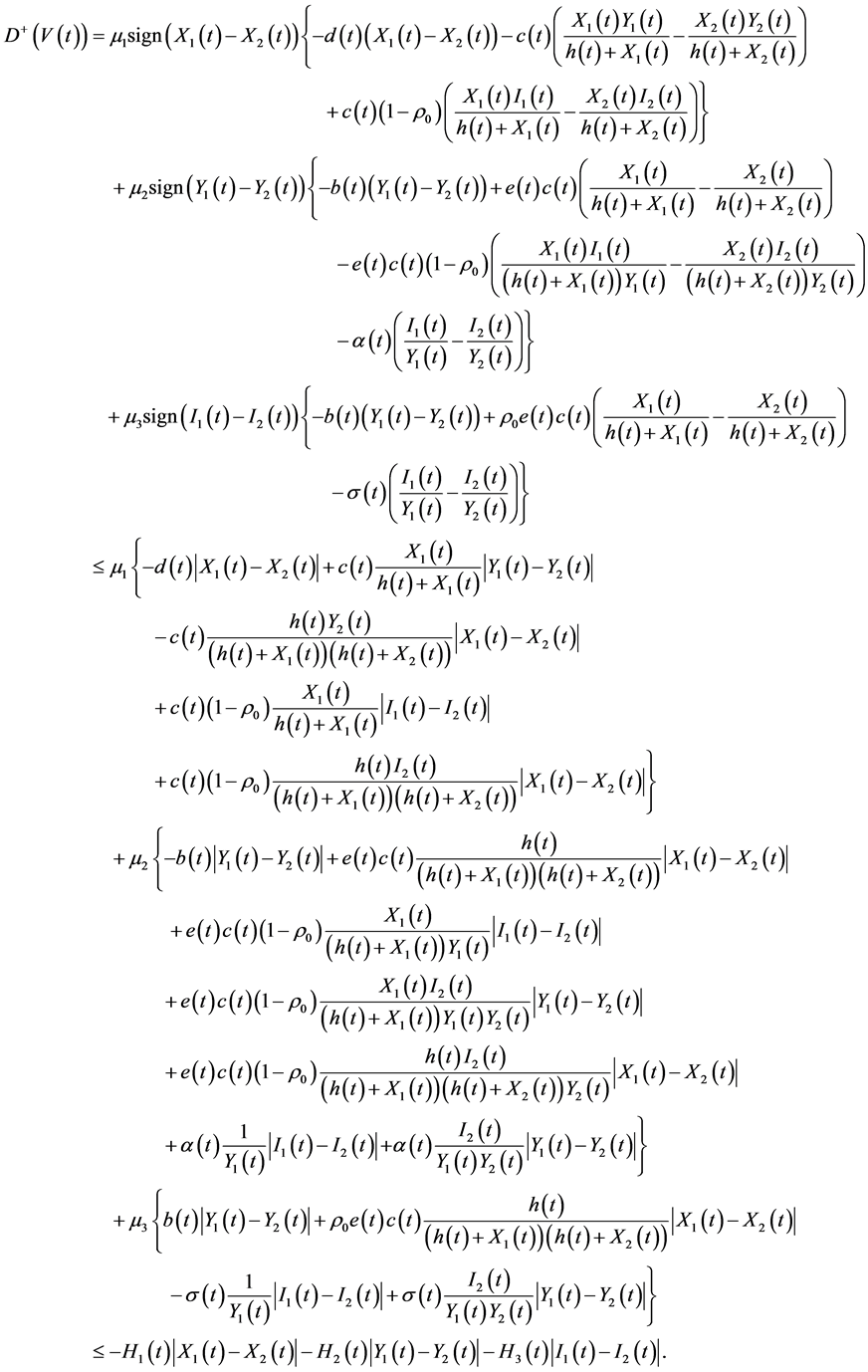
According to the condition $\underset{t\to \infty }{\lim \inf }{H}_i\left(t\right)>0\left(i=1,2,3\right)$ , there exist constants

$\varpi >0$ and $T_0>0$ such that $H_i\left(t\right)\ge \varpi \left(i=1,2,3\right)$ for all $t\ge T_0$ . Moreover, we can get that

#Math_352# (3.35)

for all $t\ge T_0$ . Integrating (3.35) from $T_0$ to $t$ , we can see

$\begin{array}{l}V\left(t\right)-V\left(T_0\right)\\ \le -\varpi {\displaystyle {\int }_{T_0}^t}\left(\left|X_1\left(\theta \right)-X_2\left(\theta \right)\right|+\left|Y_1\left(\theta \right)-Y_2\left(\theta \right)\right|+\left|I_1\left(\theta \right)-I_2\left(\theta \right)\right|\right)\text{d}\theta ,\end{array}$

then we have,

$\begin{array}{r}\hfill \begin{array}{l}\varpi {\displaystyle {\int }_{T_0}^t}\left(\left|X_1\left(\theta \right)-X_2\left(\theta \right)\right|+\left|Y_1\left(\theta \right)-Y_2\left(\theta \right)\right|+\left|I_1\left(\theta \right)-I_2\left(\theta \right)\right|\right)\text{d}\theta \\ \le V\left(T_0\right)<+\infty .\end{array}\end{array}$ (3.36)

From (3.34) and system (3.33), we can obtain that $\frac{\text{d}}{\text{d}t}\left(X_1\left(t\right)-X_2\left(t\right)\right)$ , $\frac{\text{d}}{\text{d}t}\left(Y_1\left(t\right)-Y_2\left(t\right)\right)$ , $\frac{\text{d}}{\text{d}t}\left(I_1\left(t\right)-I_2\left(t\right)\right)$ are all bounded on $\left[0,\infty \right)$ .

Therefore, in view of (3.36), we obtain

$\underset{t\to \infty }{\lim }\left|X_1\left(t\right)-X_2\left(t\right)\right|=0,\underset{t\to \infty }{\lim }\left|Y_1\left(t\right)-Y_2\left(t\right)\right|=0,\underset{t\to \infty }{\lim }\left|I_1\left(t\right)-I_2\left(t\right)\right|=0.$

In other words, the system (1.2) is globally attractive. This completes the proof.

4. Numerical Simulation and Discussion

Numerical verification of the results is necessary for completeness of the analytical study. In this section, we present some numerical simulations to verify our analytical findings of system (1.2) by means of the software Matlab.

In system (1.2), let $A\left(t\right)=2+1.5\sin \left(t\right)$ , $d\left(t\right)=0.436+0.1\sin \left(t\right)$ , $c\left(t\right)=0.5+0.05\cos \left(t\right)$ , $e\left(t\right)=0.4+0.08\sin \left(t\right)$ , $h\left(t\right)=2+0.2\sin \left(t\right)$ , $\rho =0.85$ , $r\left(t\right)=0.8+0.3\sin \left(t\right)$ , $b\left(t\right)=1.5+0.1\sin \left(t\right)$ , and $\alpha \left(t\right)=0.2+0.03\sin \left(t\right)$ . Obviously, it is easy to verify that assumptions (B1), (B2) and (B3) hold. Let $\sigma \left(t\right)=0.06+0.03\cos \left(t\right)$ , our results show that the upper threshold value $R^{\ast }=0.9934<1$ . Thus the conditions of Corollary 3.2 are satisfied, and the disease will be extinct (see Figure 1).

Increasing the infective rate $\sigma \left(t\right)$ to $0.22+0.03\cos \left(t\right)$ , we can easily get the lower threshold value $R_{\ast }=1.0441>1$ . From Corollary 3.1, we know that the disease will be permanent (see Figure 2).

Moreover, in system (1.2), let $A\left(t\right)=2+0.5\sin \left(t\right)$ , $d\left(t\right)=0.5+0.2\sin \left(t\right)$ , $c\left(t\right)=0.4+0.04\cos \left(t\right)$ , $e\left(t\right)=0.4+0.1\sin \left(t\right)$ , $h\left(t\right)=4+0.5\sin \left(t\right)$ , $\rho =0.5$ , $r\left(t\right)=5+0.4\sin \left(t\right)$ , $b\left(t\right)=2+0.2\sin \left(t\right)$ , $\alpha \left(t\right)=0.1+0.03\sin \left(t\right)$ , and $\sigma \left(t\right)=0.8+0.1\cos \left(t\right)$ . Considering system (1.2) with initial conditions (4, 0.02, 0.8), (3.2, 0.001, 2.8), (3.9, 0.001, 2.8), (3.7, 0.003, 2.6), (3.4, 0.02, 2.6), numerical simulations show that the solution curves finally converge into a closed curve in

three-dimensional space, which implies that there exists a periodic solution of system (1.2), and it is globally attractive (see Figure 3). Therefore, we conjecture that if all the conditions of theorem 3.4 hold, then system (1.2) has a periodic solution which is globally attractive. This will be left as our future consideration. Moreover, the conditions on the permanence and extinction of the infected prey species can merge into a threshold criterion and the thresholds $R_{\ast },R^{\ast }$ are obtained in Corollaries 3.1 and 3.2. However, the conditions for permanence and extinction of the model that we propose are not perfect. The threshold value has not been determined. These will be our future work for the perfection of the model.

Finally, we will perform some numerical simulations to show the importance of contact rate σ. For system (1.2), in which all the coefficients are time-dependent, we then also discuss the effect of the mean value of contact rate σ on the dyna- mics of the system. Let us fix $A\left(t\right)=2+1.5\sin \left(t\right)$ ; $d\left(t\right)=0.436+0.1\sin \left(t\right)$ , $c\left(t\right)=0.5+0.05\cos \left(t\right)$ , $e\left(t\right)=0.4+0.08\sin \left(t\right)$ , $h\left(t\right)=2+0.2\sin \left(t\right)$ , $\rho =0.85$ , $r\left(t\right)=0.8+0.3\sin \left(t\right)$ , $b\left(t\right)=1.5+0.1\sin \left(t\right)$ , $e\left(t\right)=0.2+0.1\sin \left(t\right)$ , $\alpha \left(t\right)=0.2+0.03\sin \left(t\right)$ , and $T=2\text{π}$ . As σ varies in [0.01, 0.3], we obtain the graph for the relation of the upper threshold value $R_{\ast }$ to σ (see Figure 4). This figure shows that decreasing the amplitude of periodic contact rate will reduce the risk of epidemic prevalence.

Acknowledgements

The research has been supported by The National Natural Science Foundation of China (11561004), The 12th Five-Year Education Scientific Planning Project of Jiangxi Province (15ZD3LYB031).

Cite this paper

Luo, Y.Q., Gao, S.J. and Liu, Y.J. (2017) Analysis of a Nonautonomous Eco-Epidemiological Model with Saturated Predation Rate. Applied Mathematics, 8, 252-273. https://doi.org/10.4236/am.2017.82021

References

- 1. Krishna, P.D., Chatterjee, S. and Chattopadhyay, J. (2010) Occurrence of Chaos and Its Possible Control in a Predator-Prey Model with Density Dependent Disease-Induced Mortality on Predator Population. Journal of Biological Systems, 18, 399-435. https://doi.org/10.1142/S021833901000339
- 2. Chatterjee, S., Bandyopadhyay, M. and Chattopadhyay, J. (2006) Proper Predation Makes the System Disease Free-Conclusion Drawn from an Eco-Epidemiological Model. Journal of Biological Systems, 14, 599-616. https://doi.org/10.1142/S0218339006001970
- 3. Xiao, Y. and Chen, L. (2001) Modeling and Analysis of a Predator-Prey Model with Disease in the Prey. Mathematical Biosciences, 171, 59-82. https://doi.org/10.1016/S0025-5564(01)00049-9
- 4. Xiao, Y. and Chen, L. (2001) Analysis of a Three Species Eco-Epidemiological Model. Journal of Mathematical Analysis & Applications, 258, 733-754. https://doi.org/10.1006/jmaa.2001.7514
- 5. Agarwal, M. and Pandey, P. (2008) A Stage-Structured Predator-Prey Model with Disease in the Prey. Journal of Physics: Conference Series, 96, Article ID: 012118. https://doi.org/10.1088/1742-6596/96/1/012118
- 6. Greenhalgh, D. and Haque, M. (2007) A Predator-Prey Model with Disease in the Prey Species only. Mathematical Methods in the Applied Sciences, 30, 911-929. https://doi.org/10.1002/mma.815
- 7. Chattopadhyay, J. and Arino, O. (1999) A Predator-Prey Model with Disease in the Prey. Nonlinear Analysis: Theory, Methods & Applications, 36, 747-766. https://doi.org/10.1016/S0362-546X(98)00126-6
- 8. Wang, J. and Qu, X. (2011) Qualitative Analysis for a Ratio-Dependent predatorcprey Model with Disease and Diffusion. Applied Mathematics and Computation, 217, 9933-9947. https://doi.org/10.1016/j.amc.2011.04.030
- 9. Wuhaib, S.A. and Abu Hasan, Y. (2012) A Prey Predator Model with Vulnerable Infected Prey. Applied Mathematical Sciences, 6, 5333-5348.
- 10. Zou, L., Xiong, Z. and Shu, Z. (2011) The Dynamics of an Eco-Epidemic Model with Distributed Time Delay and Impulsive Control Strategy. Journal of the Franklin Institute, 348, 2332-2349. https://doi.org/10.1016/j.jfranklin.2011.06.023
- 11. Shi, X., Cui, J. and Zhou, X. (2011) Stability and Hopf Bifurcation Analysis of an Eco-Epidemic Model with a Stage Structure. Nonlinear Analysis: Theory, Methods & Applications, 74, 1088-1106. https://doi.org/10.1016/j.na.2010.09.038
- 12. Mandal, P.S. and Banerjee, M. (2012) Deterministic Chaos vs. Stochastic Fluctuation in an Eco-Epidemic Model. Mathematical Modelling of Natural Phenomena, 7, 99-116. https://doi.org/10.1051/mmnp/20127308
- 13. Liu, X. and Wang, C. (2010) Bifurcation of a Predator-Prey Model with Disease in the Prey. Nonlinear Dynamics, 62, 841-850. https://doi.org/10.1007/s11071-010-9766-7
- 14. Li, J., Gao, W. and Sun, P. (2010) Analysis of a Prey-Predator Model with Disease in Prey. Applied Mathematics and Computation, 217, 4024-4035. https://doi.org/10.1016/j.amc.2010.10.009
- 15. Shao, Y., Li, P. and Tang, G. (2012) Dynamic Analysis of an Impulsive Predator-Prey Model with Disease in Prey and Ivlev-Type Functional Response. Abstract & Applied Analysis, 4, 1-16. https://doi.org/10.1155/2012/750530
- 16. Kang, A., Xue, Y. and Jin, Z. (2008) Dynamic Behavior of an Eco-Epidemic System with Impulsive Birth. Journal of Mathematical Analysis and Applications, 345, 783-795. https://doi.org/10.1016/j.jmaa.2008.04.043
- 17. Liu, J., Zhang, T. and Lu, J. (2012) An Impulsive Controlled Eco-Epidemic Model with Disease in the Prey. Journal of Applied Mathematics and Computing, 40, 459-475. https://doi.org/10.1007/s12190-012-0573-9
- 18. Mukherjee, D. (2010) Hopf Bifurcation in an Eco-Epidemic Model. Applied Mathematics and Computation, 217, 2118-2124. https://doi.org/10.1016/j.amc.2010.07.010
- 19. Bhattacharyya, R. and Mukhopadhyay, B. (2010) Analysis of Periodic Solutions in an Ecoepidemiological Model with Saturation Incidence and Latency Delay. Nonlinear Analysis: Hybrid Systems, 4, 176-188. https://doi.org/10.1016/j.nahs.2009.09.007
- 20. Xue, Y., Kang, A. and Jin, Z. (2008) The Existence of Positive Periodic Solutions of an Eco-Epidemic Model with Impulsive Birth. International Journal of Biomathematics, 1, 327-337. https://doi.org/10.1142/S1793524508000278
- 21. Xiao, Y. and Van Den Bosch, F. (2003) The Dynamics of an Eco-Epidemic Model with Biological Control. Ecological Modelling, 168, 203-214. https://doi.org/10.1016/S0304-3800(03)00197-2
- 22. Haque, M. (2010) A Predator-Prey Model with Disease in the Predator Species Only. Nonlinear Analysis: Real World Applications, 11, 2224-2236. https://doi.org/10.1016/j.nonrwa.2009.06.012
- 23. Zhang, J., Li, W. and Yan, X. (2008) Hopf Bifurcation and Stability of Periodic Solutions in a Delayed Eco-Epidemiological System. Applied Mathematics and Computation, 198, 865-876. https://doi.org/10.1016/j.amc.2007.09.045
- 24. Niu, X., Zhang, T. and Teng, Z. (2011) The Asymptotic Behavior of a Nonautonomous Eco-Epidemic Model with Disease in the Prey. Applied Mathematical Modelling, 35, 457-470. https://doi.org/10.1016/j.apm.2010.07.010
- 25. Zhang, Y., Gao, S. and Liu, Y. (2012) Analysis of a Nonautonomous Model for Migratory Birds with Saturation Incidence Rate. Communications in Nonlinear Science and Numerical Simulation, 17, 1659-1672. https://doi.org/10.1016/j.cnsns.2011.08.040
- 26. Haque, M., Sarwardi, S., Preston, S. and Venturino, E. (2011) Effect of Delay in a Lotka-Volterra Type Predator-Prey Model with a Transmissible Disease in the Predator Species. Mathematical Biosciences, 234, 47-57. https://doi.org/10.1016/j.mbs.2011.06.009
- 27. Teng, Z. and Li, Z. (2000) Permanence and Asymptotic Behavior of the N-Species Nonautonomous Lotka Volterra Competitive Systems. Computers & Mathematics with Applications, 39, 107-116. https://doi.org/10.1016/S0898-1221(00)00069-9
- 28. Zhang, T. and Teng, Z. (2007) On a Nonautonomous SEIRS Model in Epidemiology. Bulletin of Mathematical Biology, 69, 2537-2559. https://doi.org/10.1007/s11538-007-9231-z
- 29. Feng, X., Teng, Z. and Zhang, L. (2008) The Permanence for Nonautonomous N-Species Lotka-Volterra Competitive Systems with Feedback Controls. Rocky Mountain Journal of Mathematics, 38, 1355-1376. https://doi.org/10.1216/RMJ-2008-38-5-1355