Applied Mathematics
Vol.07 No.06(2016), Article ID:65167,13 pages
10.4236/am.2016.76051
Modeling Rift Valley Fever with Treatment and Trapping Control Strategies
Jonnes Lugoye1, Josephine Wairimu2, C. B. Alphonce1, Marilyn Ronoh2
1Univeristy of Dar es Salaam, Dar es Salaam, Tanzania
2School of Mathematics, University of Nairobi, Nairobi, Kenya

Copyright © 2016 by authors and Scientific Research Publishing Inc.
This work is licensed under the Creative Commons Attribution International License (CC BY).
http://creativecommons.org/licenses/by/4.0/


Received 8 December 2015; accepted 27 March 2016; published 30 March 2016
ABSTRACT
We consider a rift valley fever model with treatment in human and livestock populations and trapping in the vector (mosquito) population. The basic reproduction number  is established and used to determine whether the disease dies out or is established in the three populations. When
 , the disease-free equilibrium is shown to be globally asymptotically stable and the disease does not spread and when
 , a unique endemic equilibrium exists which is globally stable and the disease will spread. The mathematical model is analyzed analytically and numerically to obtain insight of the impact of intervention in reducing the burden of rift valley fever disease’s spread or epidemic and also to determine factors influencing the outcome of the epidemic. Sensitivity analysis for key parameters is also done.
Keywords:
Rift Valley Fever, Mosquito Trapping, Treatment, Rift Valley Fever Control

1. Introduction
Rift Valley Fever (RVF) is an infectious disease caused by the RVF virus of the genus Phlebovirus and family Bunyaviridae. It is transmitted between animal species, including cattle, sheep, goats, and camels, primarily through the bite of the female mosquito, usually Aedes or Culex [1] . Gaff [2] formulated an epidemiological model of RVFV determining how to reduce egg classes of mosquitoes. Clements [3] modeled the distribution of two species of mosquitoes (Aedes aegypti and Culex pipiens complex) and showed that distribution of vectors had biological and epidemiological significance in relation to disease outbreak hotspots, and provided guidance for the selection of sampling areas for RVF vectors during inter-epidemic periods. Fischer in [4] studied the transmission potential of Rift Valley Fever virus in Netherlands by developing a mathematical model to determine the initial growth and Floquet ratios which were indicators of the probability of an outbreak and persistence in a periodic changing environment caused by seasonality. Their result showed that several areas of Netherlands had a high transmission potential and risk persistence of the infection [2] . The key result is that RVF virus can persist in a closed system for 10 years if the contact rate between hosts and vectors is high [5] . Meshe [6] formulated and analysed a mathematical model described by a system of non-linear ordinary differential equations to gain insight on the dynamics of RVF in mosquito, livestock and human hosts. The disease’s threshold was computed and used to investigate the local stability of the equilibria and infer the behaviour of the disease. Tianchan et al. [7] developed a mathematical model incorporating the effect of space into the mathematical model of RVF to study the effect of the virus spread as affected by the movements of livestock, human and mosquitoes. The simulated results showed that different geographic spaces have a great effect on the spread of the pathogen and the disease in general. [8] presented the mathematical model for Rift Valley fever (RVF) transmission in cattle and mosquitoes by extending the existing models for vector-borne diseases to include an asymptomatic host class and vertical transmission in vectors. RVF remains a threat to livestock keepers and nations where the disease is occurring due to its major economic implications through the costs of the measures taken at individual, collective and international levels to prevent or control infections and disease outbreaks [9] . In this study we extend the work of [6] by incorporating the aspect of control in the modelling transmission dynamics of RVF in humans and animals, by answering the question: How does trapping of mosquitoes and/or treatment of humans and animals or both affect the spread of the disease?
The rest of the paper is arranged as follows. In Section 2, we formulate the mathematical model and establish the basic properties of the model. In Section 3, we compute the basic reproduction number herein referred to as the effective reproduction number, and determine the local and global stability of the Disease Free equilibrium. In Section 4, we establish the existence and stability of the Endemic Equilibrium. In Section 5, we have sensitivity analysis with its interpretation. Section 6 has numerical simulation and Section 7 is the conclusion.
2. Model Formulation
In this model we divide the three populations into the susceptible,  and infected,
  classes, for
  for, human (h), livestock (l) and mosquitoes (m), respectively. The three susceptible populations become infected via an infectious mosquito bite at per capita rates
 . The newborns in each category are recruited at the per capita birth rate of
  and hosts either die naturally or owing to the disease at per capita rates
  and
and , respectively. Treatment in livestock is introduced at a constant rate
 ; treatment in humans at a constant rate
  and trapping in mosquito at a constant rate
  resulting in the classes of treated livestock
 , treated humans
  and trapped mosquito
 . We assume that treated human and livestock recover at a constant rate
  respectively and return to the susceptible class again. The susceptible vector is trapped at a constant rate
 . Since a population dynamics model is considered, all the state variables and parameters are assumed to be non-negative, with as SI framework. The model assumes that individuals mix homogeneously in the human and livestock population where all individuals have equal chance of getting the infection if they come into contact with infectious mosquitoes and that transmission of the infection occurs with a standard incidence. It is the assumption of the model that there is natural mortality and disease induced death for livestock and human beings, whereas mosquitoes die only naturally, thus there is no disease induced death for mosquitoes. Again the model assumes that the individuals infected with rift valley from all three populations do not recover naturally. The schematic diagram is given below
 (1)
(1)
with initial conditions,  The force of infections
are given by  The parameters, β1, β2, β3, and β4 are the trans-
mission rates. Adding equations system 1, we have
 . (2)
. (2)
2.1. Model Analysis
In this section, we carry out stability analysis of the model (1). The model properties are employed to establish criteria for positivity of solutions and well-possessedness of the system.
2.1.1. Invariant Region
In this section a region in which solutions of the model system (4.1) are uniformly bounded in a proper subset . Let
. Let  be any solution with positive initial conditions. Then from Equation (4.1) it is noted that in the absence of the disease (i.e.
 ), the total host population size is given by,

so

where  is the value evaluated at the initial conditions of the respective variables. Thus, as
  . In respect of this, all the feasible solutions of system (1) enter the region
 .
.
Hence,  is positively invariant and it is sufficient to consider solutions in
 . Furthermore, existence, uniqueness and continuation of results for system 1 hold in this region. It is clear that all solutions of model system (1) starting in
  remain in
 . Since the model monitors populations, all parameters and state variables for system 1 are assumed to be positive. The result is summarized in the following lemma.
Lemma
The region  is positively invariant for the model system (1) with initial conditions in
 .
.
2.1.2. Positivity of Solutions
Lemma
Let the initial data be ; Then the solution set
  of the system 1 is positive
 .
.
Proof From the first equation of the model system 1
 (3)
(3)
that is

integrating by the equation above gives,


 .
.
Then
 .
.
Similarly, it can be shown that the remaining eight equations of system (4.1) are also positive .
.
3. Steady State Solutions
In this section the model system (4.1) is qualitatively analysed by determining the equilibria, carrying out their corresponding stability analysis and interpreting the results. Let , be the equilibrium point of the system (1). Then, setting the right hand side of system (1) to zero, we obtain
 (4)
(4)
From the second, fourth and sixth equations of (4), we write  and
and  in terms of
 . From the sixth equation of (4) we have,

defining
 .
.
Equation (2) reduces to (3).
3.1. Disease Free Equilibrium
This solution  of 4 leads to the disease-free equilibrium point
  is given by
 (5)
(5)
3.2. The Effective Reproductive Number, Reff
In this section, the threshold parameter that governs the spread of a disease referred to as the effective reproduction number is determined. Mathematically, it is the spectral radius of the next generation matrix [10] . The equations of the system (1) are re-written starting with infective classes, to obtain
 (6)
(6)
From the system (6),  and
and  are defined as

substituting  and
and ,
,  becomes,

The partial derivatives of  and
and  with respect to
  and
and  and evaluating at the disease free point gives

 is computed and obtained as
 .
.
The eigenvalues of  are
are  and
and

The effective reproduction number  measures the average number of new infections generated by a typical infectious individual in a community when treatment and trapping strategies are in place. As we increase trapping and treatment rates,
  have the effect of increasing
  because of linearity of
  in terms of
  taking into account that, treatment and trapping are effective.
Local Stability of the Disease Free-Equilibrium
The disease-free equilibrium point is  Thus, the Jacobian matrix
  of the
system (1) is computed by differentiating each equation in the system with respect to the state variables . Hence, at the steady states the Jacobian matrix for system (1) is given by
 (7)
(7)
where ,
,  ,
,  and
and  The characteristic polynomial is given as

Using Birkhoff and Rota's theorem on the differential inequality (3) we obtain
 .
.
From the matrix (7) we note that the first, third, fourth, fifth and sixth have diagonal entries. Therefore their corresponding eigenvalues are;
 (8)
(8)
 . (9)
. (9)
With the help of mathematical software, the following characteristic equation is obtained
 (10)
(10)
 (11)
(11)

and
 .
.
If , then
  and
and  are all negative. These results are summarised with the following theorem
Theorem
The disease-free equilibrium point is locally asymptotically stable if  and unstable if
 .
.
4. The Endemic Equilibrium, E3
In the presence s of infection, that is,  , the model system (1) has a non-trivial equilibrium point,
  called the endemic equilibrium point which is given by
 , where
  from the system (4.3). In this case, the following solution is considered
 (12)
(12)
where  is derived above. Then from the equations of system (4.3) we obtain
 (13)
(13)
 (14)
(14)
 (15)
(15)
 (16)
(16)
 (17)
(17)
 . (18)
We let  and
and  then
then
 (19)
(19)
Adding the last two equations of the system and making some simplifications we obtain
 (20)
(20)
where


 .
.
The equation,  corresponds to a situation when the disease persists (endemic). In case of backward bifurcation, multiple endemic equilibrium must exist. This implies that while considering the equation (4.18) there are three cases we have to consider depending on the signs of
  and A since B is always positive. That is;
1) If  and
and  or
or , then Equation (4.18) has a unique endemic equilibrium point (one positive root) and there is no possibility of backward bifurcation.
2) If ,
,  and
and , then Equation (4.18) has two endemic equilibria (two positive roots), and thus there is the possibility of backward bifurcation to occur.
3) Otherwise, there is none.
However it is important to note that A is always positive if  and negative if
 . Hence the above explanation leads to the following theorem.
Theorem 5 The rift valley fever basic model has,
1) Precisely one unique endemic equilibrium if 
2) Precisely one unique endemic equilibrium if  and
and  or
or 
3) Precisely two endemic equilibrium if ,
,  and
and 
4) None, otherwise.
From (iii) it is observed that backward bifurcation is possible if the discriminant is set  and solve for the critical value of
 . Thus, we get

where backward bifurcation occurs for values of  lying in the range
 . The theorem below gives the condition of existence of the endemic equilibrium point,
 .
.
Theorem 5 The endemic equilibrium point,  exists if
 .
.
5. Sensitivity Analysis
Sensitivity analysis determines parameters that have a high impact on  and should be targeted by intervention strategies. We will use the approach done in [11] and Blower and Dowlatabadi, 1994 to calculate the sensitivity indices of the effective reproduction number,
 .
.
The indices are crucial and will help us determine the importance of each individual parameter in transmission dynamics and prevalence of the Rift Valley Fever Virus.
Definition 1 The normalized forward sensitivity index of a variable, u, that depends differentiably on index
on a parameter, p is defined as; 
The analytical expression for the sensitivity of  is
is  for each of the parameter p in-
volved in . We used the following parameter values to determine the sensitivity indices;


Interpretation of Sensitivity Analysis
From Table 1, it shows that when the parameters  and
and , are increased keeping other parameters constant they increase the value of
  implying that they increase the the burden of the disease among the human, animals and vector populations as they have positive indices. While the parameters
 ,
,  and
and  decrease the value of
  when they are increased while keeping the other parameters constant, implying that they decrease the burden of the disease among the human, livestock and vector populations. The specific interpretation of each parameter shows that, the most sensitive parameter is the transmission rates for susceptible cattle individuals with infection
  followed by
  transmission rates for susceptible human individuals with infection and so on as the Table 1 indicates.
6. Numerical Simulation
We carry out numerical simulations for mathematical model of rift valley fever for the set of parameters from literature as shown in Table 1. The parameter values that changed the value of  are:
are: 
 and
and .
.
We have the following simulation results (Figures 1-6). Figure 1 shows variation of the different populations for specified parameter values. As treatment rates  and
and  increase, both infected human population
  and cattle population
  rises quickly to reach maximum and then drops to a steady state. Corresponding to the rise of both human population
  and livestock population
  infective there is a drop in the susceptible human
  and livestock
  population until reaches the minimum values and then rises to a steady state. The reduction of mosquitoes
  and
and  through trapping
  of both infected and susceptible lead to reduction in infected human and animal population because the two are infected by infected mosquitoes and they do not infect each other. The simulation results depicted in Figure 2 illustrating the the endemic state with the value of
 . The results show the introduction of trapping the mosquitoes, treating human and livestock populations reduce the reproduction number from 8.60276 to 0.4782, this implies the clearance of the disease.

Table 1. Parameter values and the calculated sensitivity indices.

Figure 1. Schematic diagram for Rift Valley Fever Model with interventions.
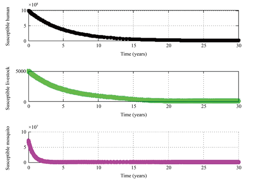
Figure 2. Population Dynamics of the rift valley fever without intervention model.

Figure 3. Effects of treatment of livestock on mosquitoes population.

Figure 4. Effects of treatment of human on mosquitoes population.

Figure 5. Effects of trapping of mosquitoes on human population.

Figure 6. Effects of trapping of mosquitoes on human population.
6.1. Variation of Different Parameters on the Dynamics of Rift Valley Fever Model with Treatment and Trapping
In this section parameters,  , and
, and  representing the treatment rate for the infected human population, treatment rate for the infected livestock population and the trapping rate for the mosquitoes population respectively were varied to determine their effect on the different model populations. When the treatment rates of livestock and human increase the infected human, livestock and mosquitoes decrease as the Figure depicts. When the trapping rate
  and
and  of the infected and susceptible mosquitoes respectively increase, the infected human and livestock decrease. This implies that endemicity of the disease among human and livestock decreases.
6.2. Discussion
The Rift Valley Model formulated in this study is well posed and exists in a feasible region where disease free and endemic equilibrium points are obtained and their stability investigated. The model has two interventions; treatment for human and livestock and trapping for mosquitoes. We have shown that disease free equilibrium exist and is locally asymptotically stable whenever its associated effective reproduction number  is less than unity, and it has a unique endemic equilibrium u when
  exceeds unity. These results have important public health implications, since they determine the severity and outcome of the epidemic (i.e. clearance or persistence of infection) and provide a framework for the design of control strategies. Analysis of the model show that in the absence of treatment of livestock and human and trapping of mosquitoes (ie.
 ) and if
 ,the epidemic will develop,but if
  it will die out. At
  (all infected human and cattle have access to treatment for human and all mosquitoes are trapped), then
 , and the epidemic will be fully controlled. The main epidemiological findings of this study include:
In the absence of treatment of human or livestock and trapping for mosquitoes:  implying that treatment failure leads the epidemic persistence. Hence the combination of treatment for livestock, humans and trapping for mosquitoes can eradicate the rift valley fever infection if
  can be reduced to below unity.
With human or livestock and trapping for mosquitoes , so; (a)
 : human or livestock treatment and trapping for mosquitoes is effective, hence elimination of infection.
7. Conclusion
In this paper, the rift valley fever model with interventions was formulated and analysed. Using the theory of differential equations, the invariant set in which the solutions of the model are biologically meaningful was derived. Boundedness of solutions was also proved. Analysis of the model showed that there exist two possible solutions, namely the disease-free point and the endemic equilibrium point. Further analysis showed that the disease-free point is locally stable implying that small perturbations and fluctuations on the disease state will always result in the clearance disease if . In the final analysis treatment and trapping interventions program will effectively control the spread of rift valley fever.
Cite this paper
Jonnes Lugoye,Josephine Wairimu,C. B. Alphonce,Marilyn Ronoh, (2016) Modeling Rift Valley Fever with Treatment and Trapping Control Strategies. Applied Mathematics,07,556-568. doi: 10.4236/am.2016.76051
References
- 1. Pepin, M., Bouloy, M., Bird, M., Kempand, B.H. and Paweska, A. (2010) Rift Valley Fever Virus (Bunyaviridae: Phlebovirus): An Update on Pathogenesis, Molecular Epidemiology, Vectors, Diagnostics and Prevention. Veterinary Research, 41, 61.
http://dx.doi.org/10.1051/vetres/2010033 - 2. Gaff, H.D., Hartley, D.M and Leahy, N.P. (2007) An Epidemiological Model of Rift Valley Fever. Electronic Journal of Di-Erential Equations, 1, 12.
- 3. Clements, A.C., Pfeifer, D.U., Martin, V. and Otte, M.J. (2007) A Rift Valley Fever Atlas for Africa. Preventive Veterinary Medicine, 2, 72-78.
http://dx.doi.org/10.1016/j.prevetmed.2007.05.006 - 4. Fischer, E., Boender, G.J. and De Koeijer, A.A. (2013) The Transmission Potential of Rift Valley Fever Virus among Livestock in the Netherlands: A Modeling Study. Veterinary Research, 44, 58.
http://dx.doi.org/10.1186/1297-9716-44-58 - 5. Métras, R., Collins, L.M., White, R.G., Alonso, S. and Chevalier, V. (2011) Rift Valley Fever Epidemiology, Surveillance, and Control: What Have Models Contributed? Vector Borne and Zoonotic Diseases, 11, 761-771.
http://dx.doi.org/10.1089/vbz.2010.0200 - 6. Mpeshe, S.C., Haario, H. and Tchuenche, J.M. (2011) A Mathematical Model of Rift Valley Fever with Human Host. Acta Biotheoretica, 59, 231-250.
http://dx.doi.org/10.1007/s10441-011-9132-2 - 7. Niu, T.C., Gaff, H.D., and Papelis, Y.E. and Hartley, D.M. (2012) An Epidemiological Model of Rift Valley Fever with Spatial Dynamics. Computational and Mathematical Methods in Medicine, 2012, Article ID: 138757.
- 8. Chitnis, N., James, M.H. and Carrie, A.M. (2013) Modelling Vertical Transmission in Vectorborne Diseases with Applications to Rift Valley Fever. Journal of Biological Dynamics, 7, 11-40.
http://dx.doi.org/10.1080/17513758.2012.733427 - 9. Otte, J.M., Nugent, R. and McLeod, A., Eds. (2004) Transboundary Animal Diseases: Assessment of Socio-Economic Impacts and Institutional Response. Volume 9, FAO, Livestock Policy Discussion Paper 9.
http://www.fao.org/ag/againfo/resources/en/publications/ - 10. Van Den, D.P. and Watmough, J. (2002) Reproduction Numbers and Sub-Threshold Endemic Equilibria for Compartmental Models of Disease Transmission. Mathematical Biosciences, 80, 29.
http://dx.doi.org/10.1016/S0025-5564(02)00108-6 - 11. Chitnis, N., Hyman, J.M. and Cushing, J.M. (2008) Determining Important Parameters in the Spread of Malaria through the Sensitivity Analysis of a Mathematical Model. Bulletin of Mathematical Biology, 70, 1272-1296.
http://dx.doi.org/10.1007/s11538-008-9299-0