Received 19 February 2014; revised 20 March 2014; accepted 28 March 2014

ABSTRACT

We study a semilinear parabolic problem with a semilinear dynamical boundary condition in an irregular domain with fractal boundary. Local existence, uniqueness and regularity results for the mild solution, are established via a semigroup approach. A sufficient condition on the initial datum for global existence is given.

Keywords:

Energy Forms, Fractal Domains, Trace Theorems, Semigroups, Semilinear Parabolic Equations

1. Introduction

In this paper we study a semilinear problem in a fractal domain with semilinear dynamical boundary conditions.

The model problem, we consider can be formally stated as follows:

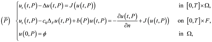
where is the (open) snowflake domain and is the union of three Koch curves (see Section 2). is a non linear function from a subset of into; m is the sum of the 2-dimensional Lebesgue measure and of the Hausdorff measure of (see Section 2.1). denotes the Laplace operator defined on (see (3.4) in Section 3), is a positive constant, is a strictly positive continuous function

in is the normal derivative across intended in a suitable sense.

More precisely, we assume that is a non linear mapping from to for any fixed locally Lipschitz i.e. Lipschitz on bounded sets in with Lipschitz constant restricted to satisfying a suitable growth condition (see condition (g)) in Section 4). Examples of this type of non linearity include e.g. which occurrs in combustion theory (see [1] ) and in the Navier Stokes system (see [2] ).

Problem presents a non linear dynamical boundary condition (known also as Venttsel’ boundary condition [3] ). Problem models a fluid diffusion within a semipermeable membrane and heat flow subject to non linear cooling on the boundary (see [4] [5] ). The literature on boundary value problems with dynamical conditions is huge, we refer to [6] for a derivation of such boundary conditions and to [7] and the references listed in. All these papers deal with smooth domains. The case of irregular domains is studied in [8] - [12] .

In the present case we consider the case in which the non linearity appears both in bulk and on the boundary. We study the problem by a semigroup approach. More precisely we consider the corresponding abstract Cauchy problem:

(1.1)

where is the generator associated to the energy form introduced in (3.8), is a fixed positive real number, is a given function in. We assume that is a mapping from locally Lipschitz i.e. Lipschitz on bounded sets in; we let denote the Lipschitz constant of:

(1.2)

whenever.

A is the generator of the analytic contraction positivity preserving semigroup from into associated to. We study problem via the corresponding integral equation

(1.3)

In order to prove the existence of the solutions to (1.3) the usual way is to use a contraction argument in suitable Banach spaces see e.g. [13] . Usually the functional setting is that of an interpolation space between the domain of the generator and or the domain of a fractional power of, we refer the reader to [13] - [17] . In our fractal case we do not know the domain of We stress the fact that it is not neither known a characterization of the domain of the fractal Laplacian To overcome this difficulty we adapt the abstract approach in [18] to prove local existence and uniqueness results for the mild solution. The key tool in [18] is an assumption on the estimate of the semigroup as a bounded operator from to (see (2.1) in [18] ). In the present case we take into account that our problem has a probabilistic interpretation [19] ; this, in turn, allows us to deduce an analogue estimate of as a bounded map from to see (3.15). We then deal with the strong formulation of the B.V.P. satisfied by the mild solution, which is of course of great interest in the applications, actually we prove that the solution of problem solves in a suitable sense Problem see Theorems 5.1 and 5.2.

The layout of the paper is the following in Section 2 we recall the preliminaries on the geometry and the functional spaces. In Section 3 we consider the energy forms and the associated semigroups. In Section 4 we consider the abstract Cauchy problem and we prove local and global existence results. Finally in Section 5 we prove that the solution of the abstract Cauchy problem solves problem in a suitable sense.

2. Preliminaries

2.1. Geometry

In the paper we denote by points in, by the Euclidean distance and by the Euclidean balls. By the Koch snowflake F, we will denote the union of three coplanar Koch curves (see [20] ), and as shown in Figure 1. We assume that the junction points, and are the vertices of a regular triangle with unit side length, i.e.. From now on we assume that a clockwise orientation is given on.

The Hausdorff dimension of the Koch snowflake is given by. This fractal is no longer self-similar

(and hence, not nested).

One can define, in a natural way, a finite Borel measure supported on by

(2.1)

where denotes the normalized -dimensional Hausdorff measure, restricted to,.

The measure has the property that there exist two positive constants, such that

(2.2)

where and where denotes the Euclidean ball in. As is supported on, it

is not ambiguous to write in (2.2) in place of. In the terminology of the following section we say that is a d-set with according to [21] .

Remark 2.1. The Koch snowflake can be also regarded as a fractal manifold (see [22] ).

We denote by the (open) snowflake domain.

2.2. Functional Spaces

By we denote the Lebesgue space with respect to the Lebesgue measure on subsets of, which will be left to the context whenever that does not create ambiguity. By we denote the Hilbert space of square summable functions on with respect to the invariant measure Let be a closed set of, by we denote the space of continuous functions on, by we denote the space of continuous functions vanishing on. Let be an open set of, by, where we denote the usual (possibly fractional) Sobolev spaces (see [23] ); is the closure of, (the infinitely differentiable functions with compact support on), with respect to the -norm.

We now recall a trace theorem.

For in, we put

(2.3)

at every point where the limit exists. It is known that the limit (2.3) exists at quasi every with respect to the -capacity [24] .

Definition 2.2. Let be a closed non-empty subset. It is a d-set if there exists a Borel

measure with such that for some constants and

(2.4)

Such a is called a d-measure on.

Proposition 2.3. The set is a d-set with. The measure is a d-measure.

See [22] and [25] .

Throughout the paper will denote possibly different constants.

We now come to the definition of the Besov spaces.

Actually there are many equivalent definitions of these spaces see for instance [21] and [26] . We recall here the one which best fits our aims and we will restrict ourselves to the case,; the general setting being much more involved see [18] . By we denote the space of functions

where

Theorem 2.4. Let then is the trace space to F of in the following sense:

1) is a continuous linear operator from to,

2) there is a continuous linear operator from to such that is the identity operator in.

For the proof we refer to Theorem 1 of Chapter VII in [21] , see also [26] .

From now on we denote by.

3. Energy Forms and Semigroups Associated

3.1. The Energy Form E

In Definition 4.5 of [22] a Lagrangian measure on and the corresponding energy form as

(3.1)

with domain have been introduced. The domain, which is a Hilbert space with norm

(3.2)

has been characterized in terms of the domains of the energy forms on (see [22] Theorem 4.6).

In the following we will omit the subscript, the Lagrangian measure will be simply denoted by and we will set, an analogous notation will be adopted for the energies.

In the following we shall also use the form which is obtained from by the polarization identity:

(3.3)

It can be proved as in Proposition 3.1 of [22] , that:

Proposition 3.1. In the previous notations and assumptions the form with domain is a regular Dirichlet form in and the space is a Hilbert space under the intrinsic norm (3.2).

For the definition and properties of regular Dirichlet forms we refer to [27] . We now define the Laplace operator on. As is a regular Dirichlet form on, with domain dense in, there exists (see Chap. 6, Theorem 2.1 in [28] ) a unique self-adjoint, non positive operator on―with domain dense in―such that

(3.4)

Let denote the dual of the space. We now introduce the Laplace operator on the fractal as a variational operator from by

(3.5)

for and for all where is the duality pairing between and. We use the same symbol to define the Laplace operator both as a self-adjoint operator in (3.4) and as a variational operator in (3.5). It will be clear from the context to which case we refer.

In the following we denote by

(3.6)

defined in where denotes a strictly positive continuous function in is also a Dirichlet form in

Consider now the space of functions

(3.7)

The space is non trivial. We now introduce the energy form

(3.8)

defined on the domain. In the following we denote by the Lesbegue space with respect to the measure with

(3.9)

By, we will denote the corresponding bilinear form

(3.10)

defined on.

Proposition 3.2. The form defined in (3.8) is a Dirichlet form in and the space is a Hilbert space equipped with the scalar product

(3.11)

We denote by the norm in associated with (3.11) , that is

(3.12)

Resolvents and Semigroups Associated to Energy Forms

As is a closed bilinear form on, with domain dense in, there exists (see chap. 6 Theorem 2.1 in [28] ) a unique self-adjoint non positive operator on, with domain dense in, such that

(3.13)

Moreover in Theorem 13.1 of [27] it is proved that to each closed symmetric form a family of linear operators can be associated with the property

and this family is a strongly continuous resolvent with generator A, which also generates a strongly continuous semigroup

With similar arguments it can be proved that there exists a nonnegative self-adjoint operator with

domain such that we denote by the

strongly continuous semigroup associated to on

Proposition 3.3. Let and be the semigroups generated by the operator A and respectively, associated to the energy form in (3.13) and in (3.6). Then and are analytic contraction positive preserving semigroups in and respectively.

Proof. The contraction property follows from Lumer Phillips Theorem on dissipative operators (Chapter 1 Theorem 4.3 in [16] ). In order to prove the analyticity it will be enough to prove that there exists a positive

such that (see Proposition 3 Section 6 in Chapter XVII in [29] ). Moreover since

the semigroup is Markovian it is positive preserving. □

Remark 3.4. It is well known that the symmetric and contraction analytic semigroup uniquely determines analytic semigroups on the space see (Theorem 1.4.1 [30] ) which we still denote by and by its infinitesimal generator.

Let denote the spectral dimension of [31] [32] . By Theorem B3.7 in [33] one can prove

Proposition 3.5. For any is a bounded operator and

(3.14)

Proof. The result follows by using the equivalence between (3.14) and Nash inequality. Actually it holds that for any

(see [34] ). □

From Theorem 2.11 in [19] the following estimate on the decay of the heat semigroup holds.

Proposition 3.6. There exists a positive constant such that

We will consider the case and.

We remark that this property is called supercontractivity ( see e.g. [30] ).

From now on we set for

We recall that for every , and

From interpolation result theory (see e.g. [35] ), it can be proved that for every

with

(3.15)

where and

In particular we will often use that is bounded from with

with and

Taking into account 2.6 and we obtain

4. The Abstract Cauchy Problem: Local and Global Existence

We study the solvability of the Cauchy problem:

(4.1)

where is the generator associated to the energy form introduced in (3.8), is a fixed positive real number, is a given function in. We assume that is a mapping from locally Lipschitz i.e. Lipschitz on bounded sets in; we let denote the Lipschitz constant of:

(4.2)

whenever. We also assume that. This assumption is not necessary in all that follows but it simplifies the calculations (see [18] ). In order to prove the local existence theorem we make the following assumption on the growth of when

we note that for and

Let. Following the approach in Theorem 2 in [18] and adapting the proof of Theorem 5.1 in [8] we have:

Theorem 4.1. Let condition (g) hold. Let be sufficiently small, if and

(4.3)

There is a and a unique

with and satisfying for every:

(4.4)

with the integral being both an -valued and -valued Bochner integral.

The claim of the Theorem is proved by a contraction mapping argument on suitable spaces of continuous functions with values in Banach spaces. We adapt the proof of Theorem 5.1 in [8] to the new functional setting and for the reader’s convenience we recall it.

Proof. Let be the complete metric space defined as follows

(4.5)

equipped with the metric

Since condition (g) holds we choose such that for

For, let. By using arguments similar to those used in the proof of Lemma 2.1 of [36] we can prove that and of course . We now prove that

(4.6)

Taking into account (4.3) there exists such that for all.

from (4.5) we have that

where thus choosing (4.6) is proved. It remains to prove

that, for a suitable choice of is a contraction.

Therefore we have

We consider now It holds

In order to prove that it is a contraction it’s enough to choose such that and

. □

Remark 4.2. If then Thus condition (g) is satisfied for

with.

Since is an analytic semigroup on both and from Corollary 2.1 in [18] , the following regularity result holds (see also Theorem 5.3 in [8] ).

Theorem 4.3. Under the assumptions of Theorem 4.1 we have.

a) The solution can be continuously extended to a maximal interval as a solution of (4.4), until.

b)

and satisfies

i.e. it is a classical solution.

Proof. As to the proof of condition a), we follow Theorem 4.2 in [18] . From the proof of Theorem 4.1 it turns out that the minimum existence time for the solution to the integral equation is as long as (see also Corollary 2.1. in [18] ).

To prove that the mild solution is classical we use the classical regularity results for linear equations (see e.g. Theorem 4.3.4. in [13] ) by proving that is Hölder continuous on into for any fixed Taking into account the local Lipschitz continuity of it is enough to show that is H continuous on into. Let we set if we prove that

then, as due to the uniqueness of the solution of (4), then

for every hence is a classical solution (see claim b). Let Since is an analytic semigroup, is continuosly differentiable on, hence Hölder continuous with any exponent. It is enough to show that is Hölder continuous.

For is a bounded operator in and from Theorem 11.3 and 12.1 in [37] there exists a constant c such that

Now let then

Hence,

If we choose it follows As to the function it holds

Hence Therefore if is Hölder continuous on with exponent. □

We now give a sufficient condition on the initial datum in order to obtain a global solution adapting Theorem 3 (b) in [38] see also Theorem 5.4 in [8] .

Theorem 4.4. Let condition (g) hold. Let a.e. and is sufficiently small, then there exists a nonnegative which is a global solution of (4.4).

Proof. Since, from (3.15) it follows that is a bounded operator from into with

hence

by choosing sufficiently small from Theorem 4.1 there exists a local solution of (4.4), . Furthermore from Theorem 4.1 and . From Theorem 4.3 (a) to show that is a global solution it is enough to show that is bounded for every We will prove that is bounded for every

and we will use the notations of the proof in Theorem 4.1.

Let is a continuous non decreasing function with which satisfies

if and then can never equal If it did we would have i.e. which is false. This proves that for sufficiently small must remain bounded. □

5. Strong Interpretation and Regularity Results

Theorem 5.1. Let be the solution of problem. Then we have for every fixed

and for every

(5.7)

where, is the inward “normal derivative”, to be defined in a suitable sense. Moreover

Proof. By proceeding as in Theorem 6.1 of [39] and taking into account that we obtain for each

(5.8)

from this we deduce and, since the right hand-side belongs to we deduce that hence

where

here the Laplacian is intended in the distributional sense. By proceeding as in (3.26) of [40] [41] we prove that,

for every fixed, the normal derivative is in the dual of the space, where and

(5.9)

for every and every and by proceeding as in 6.1 of [39] we prove that

.

Let be an arbitrary function in, for every fixed we multiply Equation (4.1) in and we integrate over

(5.10)

the left hand-side of (5.10) can be written as:

from (3.13) we deduce

(5.11)

(5.12)

taking into account that from (5.9), we have

from (5.11) we have

by proceeding as in Section 6.1 of [39] it can be proved that

and the boundary condition holds in that is

(5.13)

As a consequence of Theorem (5.1) the solution of problem is the solution of the following problem. For every,

Theorem 5.2. Let be the strict solution of problem Then for every

Proof. For every we consider the weak solutions and of the following auxiliary problems

(5.14)

(5.15)

The regularity of follows from the regularity of and since

(5.16)

We note that for every (see Corollary 3.3 in [42] ) thus in particular Since is a quasicircle from Theorem 2.7 in [43] it is also a non-tangentially accessible domain (N.T.A.), this implies that it is regular for the Dirichlet problem (5.14) in the sense of Jerison and Kenig (see Definition 2.12 in [43] ); this yields in particular that As to the regularity of taking into

account that from Theorem 1.3 in [44] part B, it follows that this concludes

the proof.

Acknowledgements

The authors have been supported by the Gruppo Nazionale per l’Analisi Matematica, la Probabilit e le loro Applicazioni (GNAMPA) of the Istituto Nazionale di Alta Matematica (INdAM).

References

- Beberns, J. and Eberly, D. (1989) Mathematical Problems from Combustion Theory. Applied Mathematical Sciences, 83, Springer Verlag, NewYork.
- Giga, Y. (1986) Solutions for Semilinear Parabolic Equations in
![]() and Regularity of Weak Solutions of the Navier Stokes System. Journal of Differential Equations, 62, 186-212. >http://html.scirp.org/file/11-7402218x492.png" class="200" /> and Regularity of Weak Solutions of the Navier Stokes System. Journal of Differential Equations, 62, 186-212. http://dx.doi.org/10.1016/0022-0396(86)90096-3
and Regularity of Weak Solutions of the Navier Stokes System. Journal of Differential Equations, 62, 186-212. >http://html.scirp.org/file/11-7402218x492.png" class="200" /> and Regularity of Weak Solutions of the Navier Stokes System. Journal of Differential Equations, 62, 186-212. http://dx.doi.org/10.1016/0022-0396(86)90096-3 - Venttsel, A.D. (1959) On Boundary Conditions for Multidimensional Diffusion Processes. Teoriya Veroyatnostei i ee Primeneniya, 4, 172-185, English Translation: Theory of Probability and Its Application, 4, 164-177.
- Coclite, G.M., Goldstein, G.R. and Goldstein, J.A. (2009) Stability of Parabolic Problems with Nonlinear Wentzell Boundary Conditions. Journal of Differential Equations, 246, 2434-2447. http://dx.doi.org/10.1016/j.jde.2008.10.004
- Evans, L.C. (1977) Regularity Properties for the Heat Equation Subject Non Linear Boundary Constraints. Nonlinear Analysis: Theory, Methods & Applications, 1, 593-602. http://dx.doi.org/10.1016/0362-546X(77)90020-7
- Goldestein, R.G. (2006) Derivation and Physical Interpretation of General Boundary Conditions. Advances in Differential Equations, 11, 57-480.
- Favini, A., Goldestein, R.G. and Romanelli, S. (2002) The Heat Equation with Generalized Wentzell Boundary Condition. Journal of Evolution Equations, 2, 1-19.
- Lancia, M.R. and Vernole, P. (2012) Semilinear Evolution Transmission Problems across Fractal Layers. Nonlinear Analysis: Theory, Methods & Applications, 75, 4222-4240. http://dx.doi.org/10.1016/j.na.2012.03.011
- Lancia, M.R. and Vernole, P. (2013) Semilinear Fractal Problems: Approximation and Regularity Results. Nonlinear Analysis: Theory, Methods & Applications, 80, 216-232. http://dx.doi.org/10.1016/j.na.2012.08.020
- Lancia, M.R. and Vernole, P. (2014) Semilinear Evolution Problems with Ventcel-Type Condition on Fractal Boundaries. International Journal of Differential Equations, 2014, Article ID: 461046. http://dx.doi.org/10.1155/2014/461046
- Lancia, M.R. and Vernole, P. (2014) Venttsel’ Problems in Fractal Domains. Journal of Evolution Equations, Published Online. http://dx.doi.org/10.1007/s00028-014-0233-7
- Warma, M. (2012) Regularity and Well-Posedness of Some Quasi-Linear Elliptic and Parabolic Problems with Nonlinear General Wentzell Boundary Conditions on Nonsmooth Domains. Nonlinear Analysis: Theory, Methods & Applications, 75, 5561-5588. http://dx.doi.org/10.1016/j.na.2012.05.004
- Lunardi, A. (1995) Analytic Semigroups and Optimal Regularity in Parabolic Problems. Progress in Nonlinear Differential Equations and Their Applications, 16, Birkäuses Verlag, Basel.
- Cazenave, T. and Haraux A. (1998) An Introduction to Semilinear Evolution Equations. Oxford Science Publications, Oxford.
- Henry, D. (1981) Geometric Theory of Semilinear Parabolic Equations. Lecture Notes in Mathematics, 840, Springer-Verlag, Berlin.
- Pazy, A. (1983) Semigroup of Linear Operators and Applications to Partial Differential Equations. Applied Mathematical Sciences, 44, Published Online. http://dx.doi.org/10.1007/978-1-4612-5561-1
- Tanabe, H. (1979) Equations of Evolution. Pitman, London.
- Weissler, F.B. (1980) Local Existence and Nonexistence of Semilinear Parabolic Equations in Lp. Indiana University Mathematics Journal, 29, 79-102. http://dx.doi.org/10.1512/iumj.1980.29.29007
- Kumagai, T. (2000) Brownian Motion Penetrating Fractals. Journal of Functional Analysis, 170, 69-92. http://dx.doi.org/10.1006/jfan.1999.3500
- Falconer, K. (1990) The Geometry of Fractal Sets. 2nd Edition, Cambridge Univ. Press, Cambridge.
- Jonsson, A. and Wallin, H. (1984) Function Spaces on Subset of Rn. Part 1, Mathematics Reports, 2, Harwood Academic Publishers, London.
- Freiberg, U. and Lancia, M. R. (2004) Energy Form on a Closed Fractal Curve. Zeitschrift für Analysis und ihre Anwendungen, 23, 115-135. http://dx.doi.org/10.4171/ZAA/1190
- Necas, J. (1967) Les mèthodes directes en thèorie des èquationes elliptiques. Masson, Paris.
- Adams D.R. and Hedberg D.R. (1966) Function Spaces and Potential Theory. Springer-Verlag, Berlin.
- Mosco, U. and Vivaldi, M.A. (2003) Variational Problems with Fractal Layers. Rendiconti della Accademia nazionale delle scienze detta dei XL.: Memorie di matematica e delle sue applicazioni, 27, 237-251.
- Triebel, H. (1997) Fractals and Spectra Related to Fourier Analysis and Function Spaces. Monographs in Mathematics, 91, Birkhäuser, Basel.
- Fukushima, M., Oshima, Y. and Takeda, M. (1994) Dirichlet Forms and Symmetric Markov Processes. de Gruyter Studies in Mathematics, 19, W. de Gruyter, Berlin. http://dx.doi.org/10.1515/9783110889741
- Kato, T. (1977) Perturbation Theory for Linear Operators. 2nd Edition, Springer, Berlin.
- Dautray, R. and Lions, J.L. (1988) Mathematical Analysis and Numerical Methods for Science and Technology. 2, Springer-Verlag, Berlin.
- Davies, E.B. (1989) Heat Kernels and Spectral Theory. Cambridge Univ. Press, Cambridge.
- Fukushima, M. and Shima, T. (1992) On a Spectral Analysis for the Sierpinski Gasket. Potential Analysis, 1, 1-35. http://dx.doi.org/10.1007/BF00249784
- Rammal, R. and Tolouse G. (1983) Random Walks on Fractal Structures and Percolation Clusters. Journal de Physique Lettres, 44, 13-22. http://dx.doi.org/10.1051/jphyslet:0198300440101300
- Kigami, J. (2001) Analysis on Fractals, Cambridge Tracts in Mathematics. 143, Cambridge University Press, Cambridge.
- Mosco, U. (1997) Variational Fractals, Dedicated to Ennio De Giorgi. Annali della Scuola Normale Superiore di Pisa, 25, 683-712.
- Bergh, J. and Löfström, J. (1976) Interpolation Spaces. Springer-Verlag, Berlin. http://dx.doi.org/10.1007/978-3-642-66451-9
- Weissler, F.B. (1979) Semilinear Evolution Equations in Banach Spaces. Journal of Functional Analysis, 32, 277-296. http://dx.doi.org/10.1016/0022-1236(79)90040-5
- Komatsu, H. (1966) Fractional Powers of Operators. Pacific Journal of Mathematics, 19, 285-346. http://dx.doi.org/10.2140/pjm.1966.19.285
- Weissler, F.B. (1981) Existence and Non-Existence of Global Solutions for a Semilinear Heat Equation. Israel Journal of Mathematics, 38, 29-40.
- Lancia, M.R. and Vernole, P. (2006) Convergence Results for Parabolic Transmission Problems across Highly Conductive Layers with Small Capacity. Advances in Mathematical Sciences and Applications, 16, 411-445.
- Lancia, M.R. (2002) A Transmission Problem with a Fractal Interface. Zeitschrift für Analysis und ihre Anwendungen, 21, 113-133.
- Lancia, M.R. (2003) Second Order Transmission Problems across a Fractal Surface. Rendiconti della Accademia nazionale delle scienze detta dei XL.: Memorie di matematica e delle sue applicazioni, 27, 191-213.
- Lancia, M.R. and Vivaldi, M.A. (1999) Lipschitz Spaces and Besov Traces on Self-Similar Fractals. Rendiconti della Accademia nazionale delle scienze detta dei XL.: Memorie di matematica e delle sue applicazioni, 23, 101-106.
- Jerison, D. and Kening, C.E. (1982) Boundary Behaviour of Harmonic Functions in Nontangentially Accessible Domains. Advances in Mathematics, 46, 80-147.
- Nystrom, K. (1994) Smoothness Properties of Solutions to Dirichlet Problems in Domains with a Fractal Boundary. Doctoral Thesis, University of Umeä, Umeä.
and Regularity of Weak Solutions of the Navier Stokes System. Journal of Differential Equations, 62, 186-212. >http://html.scirp.org/file/11-7402218x492.png" class="200" /> and Regularity of Weak Solutions of the Navier Stokes System. Journal of Differential Equations, 62, 186-212.