Applied Mathematics
Vol.5 No.6(2014), Article ID:44593,14 pages DOI:10.4236/am.2014.56090
An Introduction to Paraconsistent Integral Differential Calculus: With Application Examples
João Inácio Da Silva Filho1,2
1Group of Applied Paraconsistent Logic, Santa Cecília University, Santos, Brazil
2Institute for Advanced Studies, University of São Paulo, São Paulo, Brazil
Email: inacio@unisanta.br
Copyright © 2014 by author and Scientific Research Publishing Inc.
This work is licensed under the Creative Commons Attribution International License (CC BY).
http://creativecommons.org/licenses/by/4.0/


Received 21 January 2014; revised 21 February 2014; accepted 27 February 2014
ABSTRACT
In this paper we show that it is possible to integrate functions with concepts and fundamentals of Paraconsistent Logic (PL). The PL is a non-classical Logic that tolerates the contradiction without trivializing its results. In several works the PL in his annotated form, called Paraconsistent logic annotated with annotation of two values (PAL2v), has presented good results in analysis of information signals. Geometric interpretations based on PAL2v-Lattice associate were obtained forms of Differential Calculus to a Paraconsistent Derivative of first and second-order functions. Now, in this paper we extend the calculations for a form of Paraconsistent Integral Calculus that can be viewed through the analysis in the PAL2v-Lattice. Despite improvements that can develop calculations in complex functions, it is verified that the use of Paraconsistent Mathematics in differential and Integral Calculus opens a promising path in researches developed for solving linear and nonlinear systems. Therefore the Paraconsistent Integral Differential Calculus can be an important tool in systems by modeling and solving problems related to Physical Sciences.
Keywords:Paraconsistent Logic, Paraconsistent Annotated Logic, Paraconsistent Mathematics, Paraconsistent Integral Differential Calculus

1. Introduction
The Paraconsistent Logic (PL) belongs to the class of non-classical logics and presents in its foundation some tolerances at contradiction, without invalidating the conclusions. Its extended form called Paraconsistent Annotated Logic (PAL), has in its representation an associated Lattice that allows the development of algorithmic techniques and direct applications [1] -[3] . Paraconsistent Mathematics is structured on Paraconsistent Logic (PL) and has as main purpose the study of common mathematical objects such as sets, numbers and functions, where some contradictions are allowed. The PAL treating information signals in its special form called Paraconsistent Logic with annotation of two values (PAL2v) allow extracting equations for applications in signal analysis. It is possible through a Lattice FOUR of values (Hasse Diagram), obtained in the PAL2v representation, how much the annotation (or evidences) can express the knowledge about a proposition P.
The PAL2v-Lattice [4] can be formed ordered pairs of values (m, λ), which will form the annotation. In this representation, an operator ~ is fixed: |t| ® |t| where: .
.
As seen in [3] and [4] through geometric transformations we can find a Lattice of values equivalent to an associate at PAL2v. These interpretations with PAL2-Lattice of values allow Paraconsistent mathematical calculations through equations of parameterization [4] . In x-axis, PAL2v-Lattice is possibly identified by the Certainty Degree, that is achieved by:
 (1)
(1)
where: m is Favorable evidence Degree, where .
.
λ is Favorable evidence Degree, where .
.
As seen in Figure 1 the Certainty Degree values, which belong to the set  vary in closed range −1 to +1 and are in the horizontal axis of the PAL2v-Lattice of values called “Axis of degrees of certainty”.
The Contradiction Degree (Dct) is obtained by:
 (2)
(2)
As seen in Figure 1 the resulting values of Dct belong to set Â, vary on the closed interval +1 and −1 and are exposed on the vertical axis of the PAL2v-Lattice called “Axis of contradiction degrees”.
By analyzing the PAL2v-Lattice [4] -[7] the concept of Paraconsistent logical state (eτ) can be correlated to the fundamental concept of state, as studied in physical science and then extended to the model based on Paraconsistent Logic.
 (3)
(3)
where: eτ is the Paraconsistent logical state.
DC is the Certainty Degree obtained according to the two degrees of Evidence μ and λ.

Figure 1. PAL2v-Lattice with Certainty Degree, Contradictory Degree and Paraconsistent logical signal.
Dct is the Contradiction Degree found according to the two degrees of Evidence μ and λ.
Figure 1 shows the Paraconsistent logical state eτ.
The Certainty Degree normalized [6] [8] from the Paraconsistent Logical Model is called Resulting Degree of Evidence which is calculated by:
 (4)
(4)
Likewise, the normalized Contradiction Degree from the Paraconsistent Logical Model is calculated by:
 (5)
(5)
Derivative and Newton’s Quotient
According to definition, the Derivative [9] -[12] of a function of one variable is defined as a limit process:
 . Considering there was an increase h such that:
 , the Derivative can be rewritten as:
 (6)
(6)
The equation can be written as h represents a variation of x, such that:
 (7)
(7)
Therefore, the Newton’s quotient is defined as the incremental ratio of f with respect to the variable x, at the point x.
 (8)
(8)
The PAL treating information signals in its special form called Paraconsistent Logic with annotation of two values (PAL2v) allows extracting equations for applications in signal analysis from the Newton’s quotient.
2. Paraconsistent Mathematics
With PAL2v applied in the Newton’s quotient, we can obtain all the information necessary and sufficient to effect the derivation of first and second order and apply them to physical systems with good results without ignoring the action of the infinitesimal [13] [14] .
2.1. First-Order Paraconsistent Derivative
Initially we will apply to the Newton’s quotient a factor of normalization K. This is necessary for that we can put its values within the limits of the PAL2v-Lattice, therefore:
 (9)
(9)
where: K is a normalization factor, whose action allows the equation to be done as the fundamentals of PAL2v.
With the normalization factor in Equation (9) are identified Degrees of Evidence of PAL2v annotation, such that:
 → Favorable Evidence Degree and
  → Unfavorable Evidence Degree.
From Equation (2) we have the Certainty Degree of the Newton’s quotient:
 (10)
(10)
Similarly, from the Equation (3) the Contradiction Degree of the Newton’s quotient:
 (11)
(11)
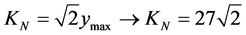
In Paraconsistent Logical Model the K value must be estimated so that the values of the degrees of evidence become established within the fundamentals of PAL2v. We can adjust this value is an equilibrium point equivalent to Planck’s constant called Paraquantum Factor of quantization, as seen in [5] and [7] .
 (12)
(12)
Be  the maximum value of the function at the considered point.
KN Paraconsistent Newton Normalization Factor.
The value of the Paraconsistent Derivative of the first-order in the physical world is obtained through reapplying the Newton Normalization Factor (KN) in the result obtained by Paraconsistent Newton’s quotient:
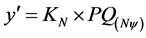 (13)
(13)
Thus, it is possible for the Paraconsistent Mathematics to be connected to the equilibrium point, defined by the Paraquantum Factor of quantization (hψ) of the PAL2v-Lattice [6] [8] . Therefore, the Paraconsistent values extracted from Newton’s quotient adjusted to Paraconsistent Logical Model depends of , that is, the increment of the variable x applied to the calculations. It is verified that the location of the Paraconsistent logical state was adjusted in the PAL2v-Lattice through the Newton Normalization Factor (KN) and identifies how it is represented any differentiable function f(x) before the mathematical procedure for obtaining the derivative. Thus, this normalization allows the function
  to be identified in the Paraconsistent Newton’s quotient, such that:
 (14)
(14)
where:  is the Favorable Evidence Degree and
  is the Unfavorable Evidence Degree. Thus, for the function
 , the Paraconsistent Newton’s quotient produces the value corresponding to the Certainty Degree (DC), which, as the fundamentals of PAL2v is obtained by Equation (12):
 (15)
(15)
Similarly, the Equation (13) the Contradiction Degree of the Paraconsistent Newton’s quotient:
 (16)
(16)
And from the Equation (4) the Evidence Degree resulting of Paraconsistent Newton’s quotient:
 (17)
(17)
And from the Equation (5) the normalized Contradiction Degree of Paraconsistent Newton’s quotient:
 (18)
(18)
2.2. Example of First-Order Paraconsistent Derivative Application
Calculate the final value of the first-order Paraconsistent Derivative of the function  in
in , with
 .
.
Resolution: Initially to form Newton Normalization Factor it is calculated the maximum value of the function  at the point considered
 , therefore, being:

The value of the Newton Normalization Factor, according to the Equation (12), is:

The Certainty Degree of Newton’s quotient is calculated by Equation (16):

The Paraconsistent Newton’s quotient is calculated according to Equation (15):


Recovering the value of Paraconsistent Derivative in the physical world by Equation (13):

Then, for these conditions of  the value of the first-order Paraconsistent Derivative of function
  in
in  is:
is: 
2.3. Paraconsistent Second-Order Derivative
Whereas the first-order Paraconsistent derivative is obtained with the calculation of the Paraconsistent Newton’s quotient Equation (9), then the Certainty Degree is:
 (19)
(19)
This first value of the Certainty Degree will be normalized by application Equation (4), turning into Favorable Evidence Degree to the second-order Derivative, so:
 (20)
(20)
Or then, (19) in (20), we have:
 (21)
(21)
The equation of Paraconsistent Newton’s quotient of the second point, or second Paraconsistent logical state, obtained into PAL2v-Lattice for second-order derivative is:
 (22)
(22)
Are identified in the Equation (22) the degrees of evidence, such that:
 → Second Favorable Evidence Degree, and
 → Second Unfavorable Evidence Degree. The Certainty Degree of second Paraconsistent logical state is calculated by:
 (23)
(23)
The second value of the Certainty Degree will be normalized, thus becoming by Equation (4) in Unfavorable Evidence Degree to the second-order Derivative of the same function f(x), so:
 (24)
(24)
Or then, (23) in (24), we have:
 (25)
(25)
For this second representation of Paraconsistent Derivative when decreases the value of  the Unfavorable Evidence degree
  approach of the Favorable Evidence Degree
 . Thus, the Paraconsistent Derivative of second order will be:
 (26)
(26)
The analysis of sequence in PAL2v will result in the Certainty degree divided by the value of the square of the increase of the variable x, so: 
The Equations (20) and (24) in (26), results in: 
Or, making (21) and (25) in (26) and rearranging, the Paraconsistent Newton’s quotient for second-order function is:
 (27)
(27)
where:  final value of the Paraconsistent Derivative function second-order.
KN is the Normalization Newton factor.
To recover and so obtain the Paraconsistent Derivative value for second-order function f(x) in actual physical universe:
 (28)
(28)
where:  is the second-order Derivative in real world.
2.4. Example of Second-Order Paraconsistent Derivative Application
Calculate the final value of the second-order Paraconsistent Derivative of the function:
 in
in , with
 .
.
For the resolution, initially is estimated the maximum function value at the point considered .
.
Therefore, being: 
The Paraconsistent Newton Normalization Factor is calculated by Equation (12):
With the Equation (27) is obtained the second-order Paraconsistent Derivative, that with:  it comes:


The value of the second-order Paraconsistent Derivative of function f(x) in actual physical universe is obtained by applying the Equation (28): 
Then, for these conditions of  the value of the second-order Paraconsistent Derivative of function
  in
in  is:
is: 
3. Paraconsistent Integral Calculus
In the calculations of Derivative every one of the Primitive functions, called here by , corresponds to a Derivative function
  [11] [14] . Is seen also that any Primitive function plus a constant positive or negative is another same Primitive Derivative, so we can establish a General Primitive function type:
The General Primitive function  is called the Indefinite Integral of the Differential
 . Therefore, the Indefinite Integral of
  is represented symbolically by:
 (29)
(29)
By other side, the Definite Integral is as an insertion of a function and extraction a number, whose value corresponds to the area between the graph of the function and the axis of x. In the calculation of Definite Integral are established the limits of integration, so the calculation is a mathematical process established between two well-defined intervals [14] [15] .
The application of the concept of Integration in a function through Paraconsistent Logical Model will be made based on the Derivative process that uses the incremental rate, or Newton’s quotient. For this condition the Paraconsistent logical State from Equation (3), which is defined in the PAL2v-Lattice by the values of the degrees of evidence, is located at one point represented by the Certainty Degree (Equation (15)) and the Contradiction Degree (Equation (16)) of Paraconsistent Newton’s quotient:
 (30)
(30)
This means that for any type function  where we can obtain the incremental ratio or Newton’s quotient, its Derivative with the adjustment with Newton normalization factor (KN) is obtained with the representation of Paraconsistent logical state onto axis of the degrees of contradiction. Figure 2 shows the location in the PAL2v-Lattice of Paraconsistent logical state
 .
.
In the method of integration in conventional mode leads to ignore the infinitesimal, as also is made in the method of limits, when considered the increase of variable x tends to zero.
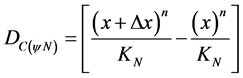
In the conventional integral method for the function  it is seen that: To a function of type
  where n is any positive integer, the initial analysis is done via the binomial theorem [14] [15] , where the term
  located on the left of the numerator of the Newton’s quotient in Equation (14), it is written as:

Subtracting  from both sides of the previous equation and dividing both sides of the equation by the increment of the variable x, and after separating in fractional terms and applying the Normalization factor of Newton, we found components of the Paraconsistent Newton’s quotient, represented by the Equation (9), as shown below:
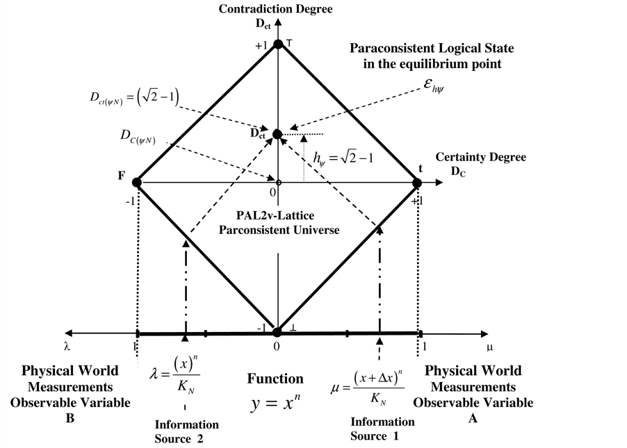
Figure 2. Location of the Paraconsistent logical state  in the point at which Newton normalization factor (KN) is used to adjust it at the equilibrium point
 .
.
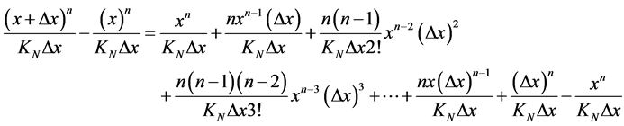 (31)
(31)
This equality Equation (31) compares Paraconsistent Newton’s quotient with the Derivative equation of conventional method before the increase of variable x tends to zero. To make the increase of variable x tends to zerothe term fractional on the right side of the Equation (31)  is eliminated. This term, which is disallowed by the conventional method by applying the binomial theorem, is identified as the Unfavorable Evidence Degree
  of PAL2v analysis. Thereby the equation expresses the limit of the function, to be described as:
 (32)
(32)
Or through another notation: 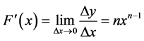 with the restriction that
 .
.
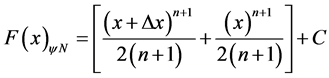
In conventional Integral method the equation of Primitive function should have adjusted their coefficient to adjust the values. Therefore, the Primitive Function of a Derivative function resulting  from conventional procedures will be:
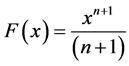 .
.
The value of the constant C is added to equation, thus obtaining the General Primitive function. And introducing the Indefinite Integral in symbolic mode, we have:
 (33)
(33)
Equations of Paraconsistent Integral Calculus
In conventional Derivative [14] before considering action of x tend to zero; the application of binomial theorem allowed Primitive function of a Derivative function had potency n – 1, such that: .
.
In the Paraconsistent Logic this mathematical process indicates that in the derivative is performed a contraction in the PAL2v-Lattice. Other action of applying the binomial theorem is that when it is made the Derivative; the eliminated term is corresponding to the degree of Unfavorable Evidence Degree  of the Paraconsistent Newton’s quotient. For the Paraconsistent Logic this mathematical process that represents the action of Derivative modifies the Certainty Degree of the Primitive function. Thereby, the Paraconsistent Newton’s quotient (Equation (14)) to the condition imposed by applying of the binomial theorem written in differential form will be:
 (34)
(34)
Therefore, for this condition, are identified:
 → Favorable Evidence Degree and
 → Unfavorable Evidence Degree.
Then, after the Derivative action, the Certainty degree, expressed by Equation (15) is:
 resulting:
 (35)
(35)
Similarly, the Derivative action also modifies the value of the Contradiction Degree (Equation (16)), that before was expressed by: . Resulting:
 (36)
(36)
To happen the Derivative action that nullifies the Unfavorable Evidence Degree  and maintains the value of the Favorable Evidence Degree
 , has an change in location of Paraconsistent logical state
  into PAL2v-Lattice. Figure 3 shows the location of Paraconsistent logical state
  after the derivative action of the Primitive function of Derivative function
 . The point where the Paraconsistent logical state
  will suffer the action of the integration process is called Paraconsistent logical state of Integral point. It is represented by
 .
.
It is verified that the Integral Paraconsistent aims to return the Paraconsistent logical state  to equilibrium point established by the Paraquantum Factor of quantization (hψ). Therefore, integral action will cause the Paraconsistent Logical State
 , that after the Derivative action was located at the Integral point
  (shown in Figure 2), it is then restored to the equilibrium point of Paraconsistent Factor of quantization, represented by
  in Figure 3. In this process of Integral Paraconsistent, which can be regarded as an anti-Derivative, when is added 1 to the n potency coefficient of x is promoted a first action in the PAL2v-Lattice expansion. Therefore, at the point of Integration
  the Favorable Evidence Degree is represented by:
 . With the expansion of the PAL2v-Lattice the Favorable Evidence Degree shall be represented by:
 . The condition for Paraconsistent logical state
  is located at the Paraconsistent equilibrium point of quantization
  is that both Degrees of evidence should exist to form the Contradiction Degree of the Paraconsistent Newton’s quotient. Therefore, as in the process of Derivative the Unfavorable Evidence Degree was made zero
 , in the integral action it is reset for your expanded value that, in this process, establishes itself as:
 .
.
At the equilibrium point, which is under the vertical axis of PAL2v-Lattice, the Contradiction Degree has its value known, such that: . Therefore, we can make the equality this known value, with the equation of Contradiction Degree where the Unfavorable Evidence Degree was reset:
 . Resulting in:
Dividing the terms of equality in the previous equation: 
Therefore, the value added to the Contradiction Degree of Paraconsistent Logic State at the integral point is
 . This value obtained in the previous equality is enough for the Paraconsistent logical state
  reach the equilibrium point of Paraconsistent Factor of quantization
  in the expanded Lattice.
After the integral action the normalized Contradiction Degree presented in Equations (5) and (18) will be:
 (37)
(37)
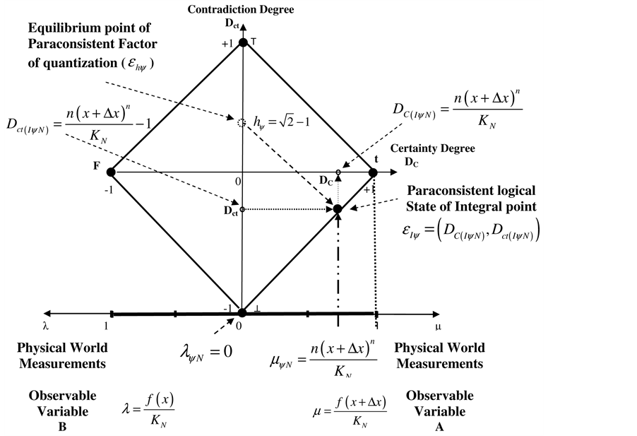
Figure 3. Location of Paraconsistent logical state of Integral point  obtained after the action process of Derivative in a Primitive function of the Derivative function.
It is verified that Paraconsistent logical state from the equilibrium point of Paraconsistent Factor of quantization  is Paraconsistent logical state of Primitive function, and it is located at the point of equilibrium determined by Paraconsistent Newton normalization Factor. Therefore the Primitive function in Paraconsistent Logical Model will be represented by the normalized Contradiction Degree of Equation (37), such that:
 (38)
(38)
where: KN is a Normalization factor of Newton, such that: 
 is the maximum value of the function at the point considered.
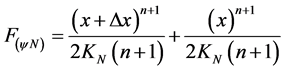
Similarly, the value of the constant C is added to the Equation (38), thus obtaining the Primitive function General:
 (39)
(39)
Figure 4 shows the Paraconsistent integral action that is expanding PAL2v-Lattice. It is verified that the Paraconsistent Integral process takes the Contradiction Degree of Paraconsistent logical state of Integral point  to the Paraconsistent logical state of equilibrium point of quantization
 .
.
Multiplies the value of KN to the result obtained in the PAL2v-Lattice, and the Primitive function final will be given by:
 (40)
(40)
The Paraconsistent Integral Undefined is presented in symbolic mode, such that:
 (41)
(41)
Thus, the calculation of the area will be:
1) For the area in the second point of the curve x = b: 
2) For the area at the first point of the curve x = a: 
The total area is calculated by:
 (42)
(42)
4. Application Examples
4.1. Example 1
Consider as a first example that is given the Derivative function  and we can find the Primitive function using the concepts of a Paraconsistent Logical Model.
Resolution: Initially, n appears in the Derivative function as: .
.
Using the Equation (39) the Primitive function by paraconsistent mode will be found:

4.2. Example 2
As second example considers that given a Derivative function from the type , we wish to find the Primitive function.
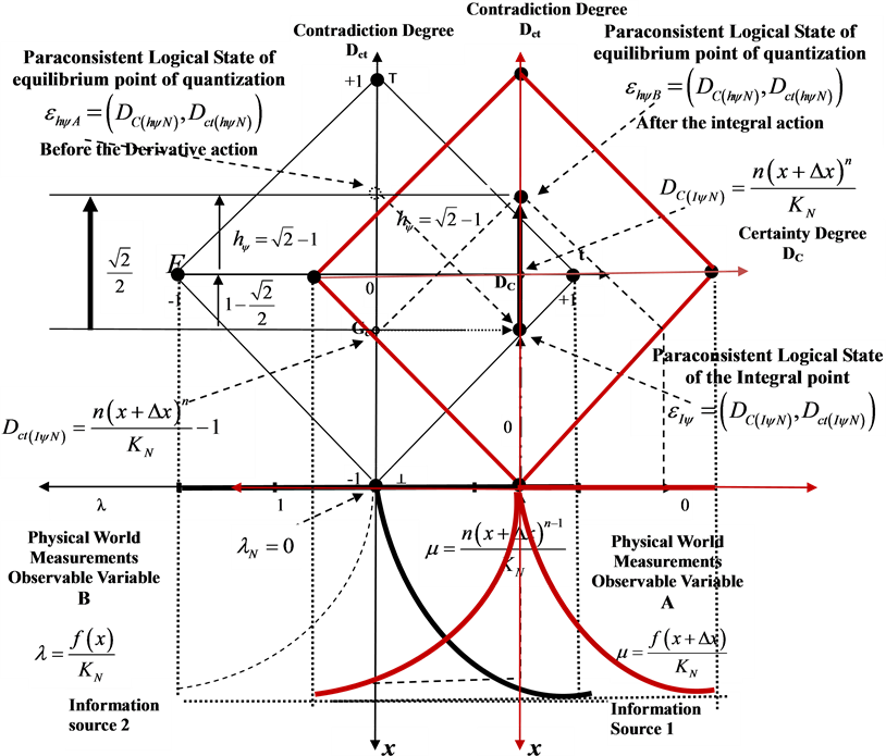
Figure 4. Final location of Paraconsistent logical state in a Paraconsistent integral process that expanding PAL2v-Lattice.
Resolution: Note that the Derivative function . Then using the Equation (41), the primitive function through the application of paraconsistent mode will be found, by:

 .
.
4.3. Example 3
Consider as a third example where we use a Paraconsistent Integral Calculus to determine the area under curve , from point
  at
at .
.
Resolution: In the resolution we can use the Equation (41) with an Increment value of variable x of :
:

For :
: 
Resulting: 
For :
: 
Resulting: 
Area calculation by the equation (42): 
 Resulting:
4.4. Example 4
Consider another example where is used the Paraconsistent Integral Calculus to determine the area under the curve  from
from  at
at .
.
Resolution: In the resolution, using the Equation (41) we can consider an Increment value of variable x: :
: 

For :
: 
Resulting: 
For :
: 
Resulting: 
With the subtraction of areas using Equation (42), we have:

4.5. Example 5
As the example 5 consider that using an increment value of the variable x of: , we wish to calculate the Paraconsistent Integral:
 .
.
Resolution: The resolution is done using the Equation (41):


For :
: 

For :
: 

We found the result of the area using the Equation (42):

Resulting: 
5. Conclusion
This article presented a Paraconsistent Mathematics that structures a method for differential and Integral Calculus using the foundations of Paraconsistent Logic applied to Newton’s quotient. The study allowed an adequacy of Differential Calculus to Paraconsistent logical model. With this, existing contradictions are accepted as inherent to a logical model based on real situations, therefore of an imperfect world. It was found that the Differential Calculus, structured in a Paraconsistent Logic that accepts contradictions, is able to dissolve the uncertainties, adding values that conventionally would be despised. Even requiring further testing involving more complex math functions the results obtained are very promising and suggest good perspectives for future applications of differential and Integral Paraconsistent Calculus.
References
- Da Costa, N.C.A. (2000) Paraconsistent Mathematics. In: Batens, D., Mortensen, C., Priest, G. and Bendegen van, J.P., Eds., I World Congress on Paraconsistency1998 Ghent, Belgium, Frontiers in Paraconsistent Logic: Proceedings, King’s College Publications, London, 165-179.
- Jas’kowski, S. (1969) Propositional Calculus for Contradictory Deductive Systems. Studia Logica, 24, 143-157. http://dx.doi.org/10.1007/BF02134311
- Da Costa, N.C.A. (1986) On Paraconsistent Set Theory. Logique et Analyse, 115, 361-371.
- Da Silva Filho, J.I., Lambert-Torres, G. and Abe, J.M. (2010) Uncertainty Treatment Using Paraconsistent Logic: Introducing Paraconsistent Artificial Neural Networks. IOS Press, Amsterdam, 328.
- Da Silva Filho, J.I. (2011) Paraconsistent Annotated Logic in Analysis of Physical Systems: Introducing the Paraquantum γψ Gamma Factor. Journal of Modern Physics, 2, 1455-1469. http://dx.doi.org/10.4236/jmp.2011.212180
- Da Silva Filho, J.I. (2012) Analysis of the Emissions Spectral line of the Paraquantum with Hydrogen Atom. Journal of Modern Physics, 3, 233-254. http://dx.doi.org/10.4236/jmp.2012.33033
- Da Silva Filho, J.I. (2012) An Introductory Study of the Hydrogen Atom with Paraquantum Logic. Journal of Modern Physics, 3, 312-333. http://dx.doi.org/10.4236/jmp.2012.34044
- Da Silva Filho, J.I. (2011) Paraconsistent Annotated Logic in analysis of Physical Systems: Introducing the Paraquantum hψ Factor of Quantization. Journal of Modern Physics, 2, 1397-1409. http://dx.doi.org/10.4236/jmp.2011.211172
- Stroyan, K.D. and Luxemburg, W.A.J. (1976) Introduction to the Theory of Infinitesimals. Academic Press, New York.
- Bell, J.L. (1998) A Primer of Infinitesimal Analysis. Cambridge University Press, Cambridge.
- Baron, M.E. (1969) The Origins of the Infinitesimal Calculus. Pergamon Press, Hungary.
- Keisler, H.J. (1976) Elementary Calculus: An Infinitesimal Approach. 1st Edition, Prindle, Weber & Schmidt, Boston.
- Diethelm, K. and Ford, N. (2004) Multi-Order Fractional Differential Equations and Their Numerical Solution. Applied Mathematics and Computation, 154, 621-640. http://dx.doi.org/10.1016/S0096-3003(03)00739-2
- Pl Tipler, A. and Llewellyn, R.A. (2007) Modern Physics. 5th Edition, W. H. Freeman and Company, New York.
- Kleene, S.C. (1952) Introduction to Metamathematics. North Holland/Van Nostrand, Amsterdam/New York.