Applied Mathematics
Vol.5 No.3(2014), Article ID:42776,19 pages DOI:10.4236/am.2014.53043
Sinogram Interpolation Method for Sparse-Angle Tomography
Department of Mathematics and Statistics, University of Helsinki, Helsinki, Finland
Email: martti.kalke@helsinki.fi
Received October 13, 2013; revised November 13, 2013; accepted November 20, 2013
ABSTRACT
In sparse-angle X-ray tomography reconstruction, where only a small number of projection images are taken around the object, appropriate sinogram interpolation has a significant impact on image quality. A novel sinogram interpolation method is introduced for extreme sparse tomographic reconstruction where only nine measured projection images are available. The sinogram is interpolated by solving characteristics of the so-called warps, which can be considered as approximation sine waves in a limited region. The numerical evidence suggests that this approach gives superior results over standard interpolation methods when the tomographic data are extremely sparse and noisy.
Keywords:Interpolation; Sparse Imaging; Tomography; Sinogram
1. Introduction
Three-dimensional (3D) X-ray imaging is typically needed for measuring the inner structures of a patient. For example, in implant dentistry where damaged or missing teeth are replaced by artificial teeth, a screw hole with accurate depth, angle and diameter is needed for the implant. The hole has to be deep enough to ensure firm attachment, but not too deep as nerves might then be damaged. This measurement cannot be based on two-dimensional (2D) images since they represent a distorted projection of the tissue. Another clinical application of 3D X-ray imaging is solving the superposition problem. Since a pixel of a 2D projection image is a sum of attenuation along the path of an X-ray, the overlapping low-contrast tissues are difficult to recognize. This can easily lead to misinterpretation and eventually cause a false diagnosis. However, in 3D imaging, the viewing angle can be chosen so that the boundaries between tissues can be accurately identified.
Lately, there has been an increasing interest in sparse-angle tomographic imaging, where fewer projection images are taken in order to reduce patient dose and scanning time. Despite that the sparse reconstruction does not offer high spatial resolution, it can offer a feasible overview on the imaging target, which extends the use of computed tomography (CT) imaging to less serious cases, like minor trauma studies or cosmetic operation planning. Moreover, sparse-angle imaging can also be used in pre-scans, where a low-resolution reconstruction is generated before the actual scan to verify patient positioning and to define optimal X-ray technique values (tube current, voltage, number of projection images) for the final scan. The pre-scan helps to optimize the patient dose and avoid re-exposures.
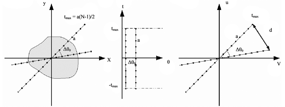
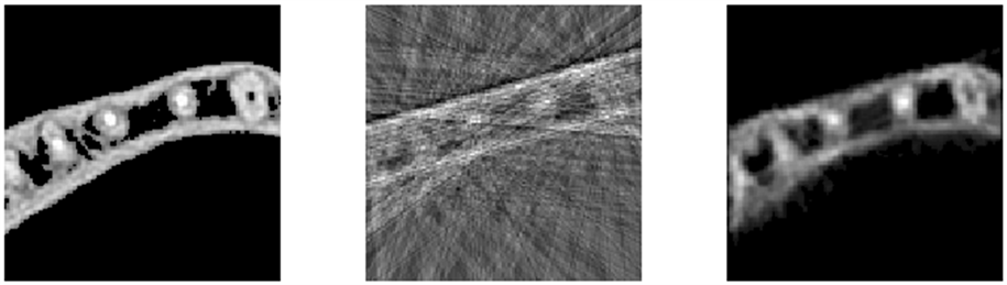
The challenge of sparse tomographic imaging is insufficient image quality caused by the inadequate number of projection images. This lack of data is illustrated in Figure 1 in the spatial, sinogram and frequency domains. In the final reconstruction, the missing information can be observed as artifacts in the 2D slice view as well as in the 3D volume view. In the slice view, the missing information generates streak artifacts (see Figures 2-4(b)),
 (a) (b) (c)
Figure 1. Representations of two projection images and their relations in (a) spatial, (b) sinogram and (c) frequency domain. The distance a is the pixel size, w is the difference of the frequency components, N is the number of pixels, Δq0 is the angular difference between the projection images and d is the maximum distance between two frequency components in adjacent columns. The relation between the spatial and the frequency domain is based on well-known Fourier Slice Theorem, which states that one projection image defines frequencies in the 2D frequency domain within a single line. This line intersects origin, it has same angle than the imaging angle and it is limited by the Nyquist frequency theorem. Books by Kak (2001) and Gonzalez (2008) provide detailed theoretical background of the Fourier Slice Theorem.
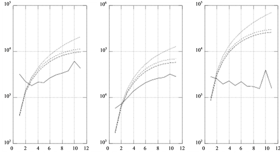
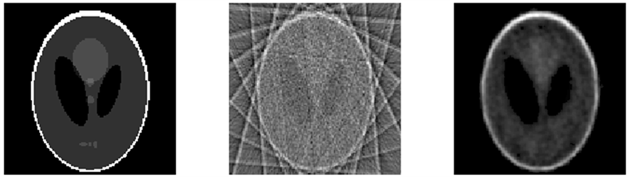
Figure 2. The FBP reconstruction of the Shepp-Logan-phantom with ![]() Gaussian noise. Upper row: (a) The original phantom, (b) reconstruction from original data and (c) SINT interpolation. Lower row: FBP reconstruction when reference interpolation methods were used; (d) linear; (e) nearest neighbor and (f) spline interpolation.
Gaussian noise. Upper row: (a) The original phantom, (b) reconstruction from original data and (c) SINT interpolation. Lower row: FBP reconstruction when reference interpolation methods were used; (d) linear; (e) nearest neighbor and (f) spline interpolation.
especially when sharp edges are present [1]. Numerical implementations of the tomographic reconstruction from sparse data are introduced for example in articles by Hyvönen et al. (2010), Rantala et al. (2006), Varjonen (2006), Siltanen et al. (2003) or Kolehmainen et al. (2003 and 2008) [2-]">7]. Moreover, the studies by Webber et al. (1999) or Cederlund et al. (2009) are illuminating examples of the capability of clinical sparse angle X-ray tomography [8,]">9]. In tomographic imaging, the reconstruction pipeline consists of three stages. The first stage is pre-processing, where the unidealities and artifacts are compensated for. In the second reconstruction stage, the 3D model is calculated based on these manipulated projection images, the known spatial relation of the gantry
 (a)
(a)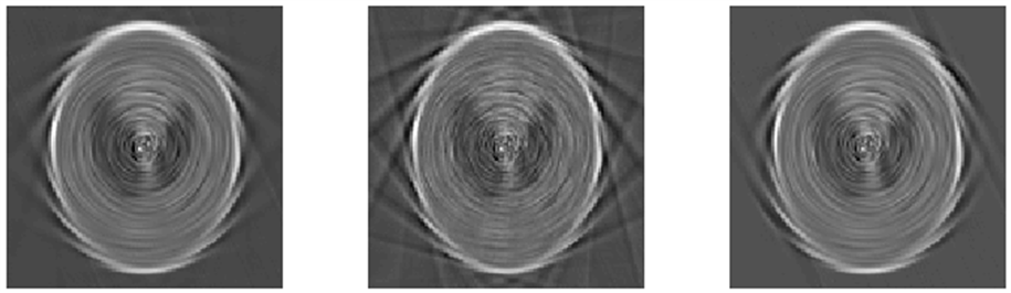 (b)
(b)
Figure 3. The FBP reconstruction of the Dental Arc-phantom with 5% Gaussian noise. Upper row: (a) The original phantom, (b) Reconstruction from original data and (c) SINT interpolation. Lower row: FBP reconstruction when reference interpolation methods were used; (d) Linear; (e) Nearest neighbor and (f) Spline interpolation.
 (a)
(a)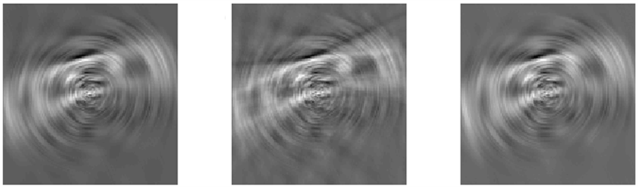 (b)
(b)
Figure 4. The FBP reconstruction of the Boxes-phantom with 5% Gaussian noise. Upper row: (a) The original phantom, (b) Reconstruction from original data and (c) SINT interpolation. Lower row: FBP reconstruction when reference interpolation methods were used; (d) Linear, (e) Nearest neighbor and (f) Spline interpolation.
(i.e. mechanical combination of the detector and the X-ray source) and the object. Finally, in the post-processing stage, the reconstruction artifacts are reduced and the clinically relevant information is emphasized. A practical and clinical overview of the reconstruction process can be found in the book by Hsieh (2009) and more theoretical approach in the book by Kak and Slaney (2001) [10,]">11].
A sinogram is a 2D representation of an X-ray CT scan, where each column represents a single row in the projection image arranged in increasing angular order. Typically, the horizontal axis represents the angle of the X-ray detector and the vertical axis, the distance from the rotation center in the detector row. Each volume element generates a sine wave in the sinogram when the X-rays are orthogonal to the detector (parallel beam geometry). Therefore, the sinogram consists of a number of overlapping sine functions, whose amplitude and phase depend on the location of the voxel and the grayvalue equals to the grayvalue of the volume element while the wavelength is constant (![]() ). As a simple example of a two-point sinogram seen in Figure 5, Figure 1 illustrates the relation between spatial and sinogram domains, and the upper row in Figure 6 is an example of a sinogram arising from sparsely sampled data. See chapter 5.11.3 in the book by Gonzalez and Woods (2008) for more information about sinogram representation [12].
). As a simple example of a two-point sinogram seen in Figure 5, Figure 1 illustrates the relation between spatial and sinogram domains, and the upper row in Figure 6 is an example of a sinogram arising from sparsely sampled data. See chapter 5.11.3 in the book by Gonzalez and Woods (2008) for more information about sinogram representation [12].
In this study, we focus on interpolating new sinogram columns without modifying the measured sinogram columns. This scenario is consistently called in this paper as sinogram interpolation. In the literature, there are also a number of other interpolation routines related to sinogram manipulation which should not be confused with the sinogram interpolation scenario. One of them is the projection image interpolation, where new values are generated between the data values to avoid Moire artifacts. This is typically handled by the standard nearestneighbor or linear interpolation [1]. Another example is needed for an interpolation routine in helical CT device for gaining uniform sampling in the azimuthal direction or metal artifact removal processes [13-]">18].
Also, the sinogram extrapolation can be used for solving the truncation problem as indicated for example by Sze and Shum (1996), Gilland et al. (2000) or Baojun and Jiang (2007) to expand the projection data in limited angle tomography [19-]">21]. Moreover, sinogram extrapolation can be used for expanding the truncated sinogram in a local tomography situation, where some of the attenuations take place outside the modeled volume (see Zamyatin and Nakanishi (2006) and references therein [22]).
Sinogram interpolation itself has been studied since the innovation of the medical CT system in the 1970’s. For example, Brooks et al. (1978) studied both interpolating new data in projection images and interpolating new projection images to attenuate Moire effects [1]. Also, Lahart (1981) studied a similar problem and used a least-squares approximation to interpolate projection images when the external shape of the object was known []">23]. However, in those days, the computational resources were very limited and therefore the spatial resolution as well as the image quality was not equivalent to today’s de-facto standards. Nevertheless, these studies illuminate the limitations of sparse and limited angle tomographic imaging and therefore can be considered as fundamental studies of sinogram estimation (see also [24-2]">7]).
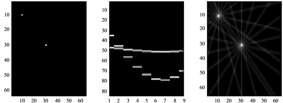
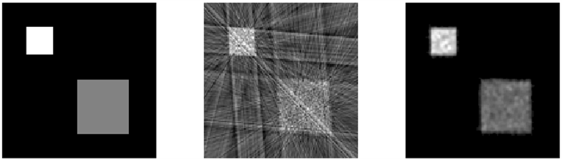
Figure 5. Example of sinogram presentation. Left is the original object with two non-zero points. Middle is the sinogram presentation of the same object when nine images are taken from 20 to 180 degree angles. Each point generates a sine shaped wave so that the amplitude is proportional to the distance between the point and the center of the object (i.e. rotation axis). Right is the reconstruction done from the projection data by using back projection algorithm.
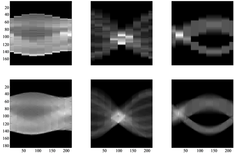
Figure 6. The original sinograms (top row) and their SINT interpolations (bottom row). Left sinogram from SheppLogan-phantom, middle from Dental Arc-phantom and right from Boxes-phantom.
Lately, there have appeared several studies on dedicated directional sinogram interpolation algorithms. For example, Zhe et al. (2003) successfully combined the Huesman algorithm with Principle Component Analysis in PET imaging, and Köstler et al. (2006) applied PDE-based methods for interpolation and the Neumann boundary condition for defining missing columns in the sinogram [28,2]">9]. In this study, about ![]() of the sinogram columns were interpolated. Similarly, in the study by Penbel et al. (2005), only
of the sinogram columns were interpolated. Similarly, in the study by Penbel et al. (2005), only ![]() of the sinogram columns were interpolated by using cumulant functions instead of linear interpolation [30]. Moreover, Bertram et al. (2004 and 2009) utilized tensors to gain directional interpolation based on sinogram data and achieved impressive results [31,]">32].
of the sinogram columns were interpolated by using cumulant functions instead of linear interpolation [30]. Moreover, Bertram et al. (2004 and 2009) utilized tensors to gain directional interpolation based on sinogram data and achieved impressive results [31,]">32].
Also, interesting approaches for sinogram interpolation in ill-posed situations are the usage of Stackgrams by Happonen (2005) and the usage of object geometry estimation for sinogram interpolation by Prince et al. (1993) [33,]">34]. The advanced general directional interpolation methods are also considered by Gerchberg (1974), Papoulis (1975) as well as La Riviere and Pan (1999) [35-3]">7]. Finally, Dong et al. (2013) introduced very promising results when combining the sinogram interpolation with the wavelet cost function [38]. For more general information about different sinogram related extrapolations and interpolations, see for example Brooks et al. (1978), Lahart (1981) or Kak and Slaney (2001) and references within [1,11,]">23].
In this paper, we introduce a new approach, called Sinogram Interpolation Technique (SINT) for estimating new sinogram columns between known, measured sinogram columns in the extremely sparse situation of only nine known sinogram columns.
This article is organized as follows: In Section 1.2, the theoretical background of the SINT method is described. Secondly, in the Section 1.3, the capability and limitations of SINT by three different numerical examples with additional noise are demonstrated. Finally, in the Section 1.4, we discuss the computational and clinical aspects of SINT and its possible future applications. Also, we analyze the failure of standard interpolation methods in extremely sparse imaging situations.
Throughout this paper, capital letters are used for matrices. Moreover, for indicating a single element in a matrix, the standard [row][column]-order is applied. For example,  indicates the element located at the
  th row and
  th column in the matrix
![]() . Notwithstanding the aforesaid, a single subscript is used for referring to columns:
. Notwithstanding the aforesaid, a single subscript is used for referring to columns:  denotes the
  th column of the matrix
![]() . Superscripts in brackets are used for additional information, like iteration round, special restrictions or relations. See Table 1 for the definition of each notation used in this work.
. Superscripts in brackets are used for additional information, like iteration round, special restrictions or relations. See Table 1 for the definition of each notation used in this work.
We systematically use the term known sinogram column for the columns that are based on actual measured X-ray projection images. The interpolated sinogram columns are called estimated columns since they are a priori unknown. Furthermore, the known sinogram columns adjacent to an estimated column are called known neighbor columns. See also Figure 7 for an illustration of this terminology.
We use the term volume for the target object and image for the projection data, although in our examples the phantoms are two-dimensional and projection images are one-dimensional. Similarly, we use the terms voxel and pixel to describe the volume and image elements to be consistent with other tomographic literature and references. Finally, in this study, we are focusing on 2D parallel beam imaging situations, where all X-rays are perpendicular to the detector. Also, we are covering only cases where the whole object is covered in each projection image, and therefore the so-called local tomography problem is excluded from this study.
2. The SINT Method
In this Section the theoretical background of the SINT method is discussed. Firstly, in Section 2.1 two new concepts, called warp and weight factor, are introduced. Secondly, in the Section 2.2 a new method for defining the grayvalues in single sinogram column located between two a priori known neighbor columns is proposed. Finally, in Section 2.3 the method is summarized and extended to cover all sinogram columns in the sinogram domain.

Table 1. Parameters used in this article.
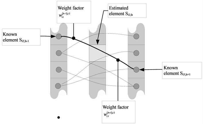
Figure 7. Outline of the warps. A single warp (thick line) connects sinogram elements ,
,  and
and  to an estimated element (light gray box). Related weight factors are also indicated.
2.1. Definitions of the Key Concepts
2.1.1. Weight Factor
In this study a sinogram is considered as a matrix  with one unknown column
 . That is
 (1.1)
(1.1)
and known projection angles corresponding to the columns of ![]() as a vector
as a vector
 (1.2)
(1.2)
where  and
and .
.
The purpose of the sinogram integration is to generate a feasible approximation for  when other columns and vector
 ![]() are known. In this method the grayvalues of each unknown sinogram element
are known. In this method the grayvalues of each unknown sinogram element  are approximated as weighted sums of nearby sinogram elements in the adjacent columns
  and
and . This can be determined in two ways, each producing the same result for
 ; either based on the column
  as
as
 (1.3)
(1.3)
or based on the column  as
as
 (1.4)
(1.4)
where  are called as the weight factors. The first upper index of weight factors indicates the known column index and the second indicates the sinogram element index in the estimated column
 . The Equations (1.3) and (1.4) clearly indicate that if the weight factors are known, then an estimate for the
  can be generated. Moreover, if the weight factors for all elements in
  are generated, an estimate for the whole sinogram column
  is gained.
The Equations (1.3) and (1.4) are combined by defining  approximation for the
  as
as
 (1.5)
(1.5)
whose solution is given by
 (1.6)
(1.6)
We end this chapter by highlighting two important identities related to weight factors. Firstly, consider a single sin wave that intersects the sinogram elements ,
,  and
and  and consists of two weight factors
  and
and . Then we have
 (1.7)
(1.7)
Secondly, because the total sum of each sinogram column is constant, the sum of all weight factors related to the same known sinogram component in columns  and
and  is always one, i.e.
 (1.8)
(1.8)
2.1.2. Warp
In extremely sparse-angle tomographic situation, the number of sine functions and their characteristic parameters (amplitude, grayvalue and phase) cannot be uniquely defined from the sinogram. For that reason, a new concept called warp is introduced. The warp can be considered as a sum of all the sine waves that intersects two sinogram elements  and
and  (see Figure 7). The most essential features of warps are:
1) Each warp has the shape of a sine wave and a wavelength of![]() . Therefore, the phase and amplitude of the warp are uniquely defined by two points.
. Therefore, the phase and amplitude of the warp are uniquely defined by two points.
2) Each warp connects two sinogram elements in known neighbors columns  and
and  to a single sinogram element in the estimated column
  by two strictly positive weight factors.
3) Each warp intersects only strictly positive sinogram elements in the whole sinogram domain.
4) All non-zero sinogram elements are associated with at least one warp and all weight factors are associated with exactly one warp.
Our interpolation strategy is to define the estimated sinogram column  by defining the amplitude, phase and so-called warp factor (will be explained in the Section 2.2) for each warp. We will show that by defining these values we can define the weight factors and thereby obtain an estimate for the sinogram column
 . Although the above warp-based approach does not completely characterize the underlying sine waves and provide an exact solution to the interpolation problem, it does give a feasible and stable approximation in limited-data situations as demonstrated in Section 1.3.
2.2. Definition of the Crucial Matrices
In this Section we will introduce three matrices to determine the connection between the warps and grayvalues of the estimated sinogram . These matrices are:
1) Matrix  to define the relation between the estimated and neighbor known sinogram elements based on the Equation (1.6)
2) Matrix ![]() to fulfill the requirement in the Equation (1.7)
to fulfill the requirement in the Equation (1.7)
3) Matrix  to limit the weight factors related to the same known sinogram based on the Equation (1.8)
We also build two temporary matrices ![]() and
and ![]() to simplify the numerical implementation. All these matrices should be generated for each sinogram column separately as described in Section 2.3.
to simplify the numerical implementation. All these matrices should be generated for each sinogram column separately as described in Section 2.3.
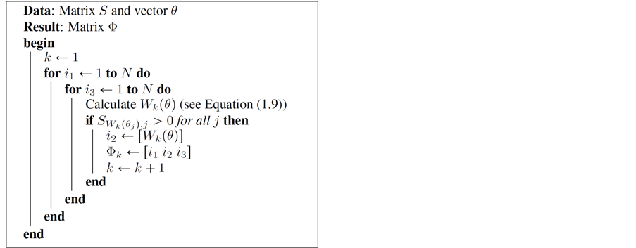
2.2.1. Warp Matrix (
The purpose of the warp matrix , where
  is the number of warps, is to simplify the creation of other matrices. The warp matrix
 ![]() defines all warps related to the estimated sinogram column
defines all warps related to the estimated sinogram column  such that each row represents a single warp as follows: The first element in the row is the row index
  of the known left point
 , the second element is the row index
  of the estimated sinogram column
  and finally the row index
  is the right known point
 .
.
To define the value  the warp function
  is defined for all angles
 ![]() based on two points in the sinogram (
based on two points in the sinogram ( and
and ) and the their angular values (
 and
and ).
).
Since the warp has the shape of a sine wave with a frequency of one and an offset of , it can be defined as
 (1.9)
(1.9)
where the amplitude ![]() and phase
and phase ![]() depend on the known angles
depend on the known angles  as follows:
 (1.10)
and
 (1.11)
where
 (1.12)
If  is for each
 , then the warp is valid (see the requirement item 3 in the Section 2.1) and finally
  where
where ![]() is the rounding operator. Because of this limitation, the height of the matrix
is the rounding operator. Because of this limitation, the height of the matrix ![]() typically smaller than
typically smaller than![]() . The procedure for generating the warp matrix
. The procedure for generating the warp matrix ![]() is described in the Algorithm 1.
is described in the Algorithm 1.
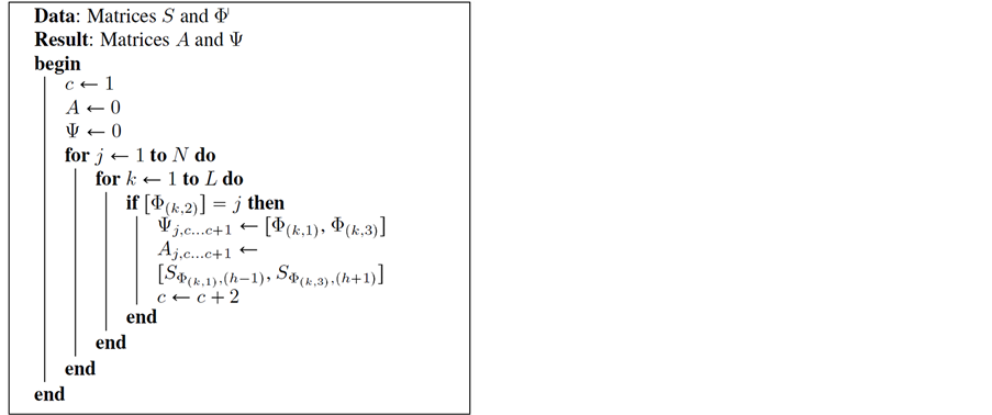
2.2.2. Relation Matrices A and (
The purpose of this phase is to define two quite similar sparse matrices; Relation Grayvalue Matrix , where and Relation Index Matrix
 . The matrix
  includes grayvalues of the known sinogram columns
  and
and ![]() consists of the corresponding row indexes. First we define the Relation Grayvalue Matrix
consists of the corresponding row indexes. First we define the Relation Grayvalue Matrix , which specifies the relations between the weight factor vector
  and the sinogram elements in the estimated column
 . The Equation (1.6) can be represented in a matrix form as
 (1.13)
where the matrix  consists of zeros and known neighbor sinogram gray values
  multiplied by
 . However, unlike in Equation (1.6), the vector
  in Equation (1.13) consists only the weight factors that are included in warps and therefore the size of the vector
  is
is . The vector
  will be called in this study as weight vector.
The relation matrix  can be constructed from the row vectors
  such that each row vector
  consists of the grayvalues of known neighbor sinogram columns that are connected to an estimated sinogram element
  by the warps as described in Section 2.2 and Figure 7. Since each weight factor is
Algorithm 1. Generation of the warp matrix F.
related to exactly one estimated sinogram element, only one non-zero value on each column is allowed. Therefore, the matrix  has the form
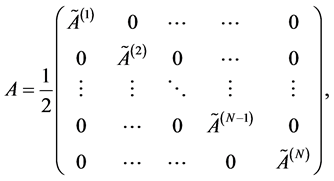 (1.14)
where ![]() are zero row vectors.
are zero row vectors.
We also need the row indexes of the known points (indicated above as  and
and ) ordered consistently with the structure of the matrix
 . Those values will be stored into matrix
 . The procedure for generating the matrices
  and
and ![]() is described in Algorithm 2.
is described in Algorithm 2.
At this point the matrices  and
and ![]() have been generated. The matrix
have been generated. The matrix  defines the relation between the estimated sinogram column and the weight factors as described in Equation (1.13). The matrix
 ![]() plays an important role in defining the eigenvector and rule matrices in the following Sections.
plays an important role in defining the eigenvector and rule matrices in the following Sections.
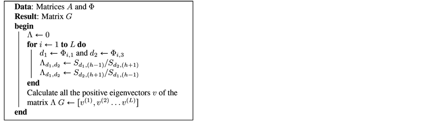
2.2.3. Eigenvector Matrix (
Having constructed the matrix  appearing in Equation (1.13), we now turn to specifying the weight vector
 . From the Equation (1.7) can be seen that
![]() (1.15)
(1.15)
where  such that

if and only if  and
and  are related to the same warp, otherwise
  and
and .
.
From the Equation (1.15) can be observed that the weight vector  is an positive eigenvector for
  related to an eigenvalue of one1. The number of feasible eigenvectors is exactly
  based on the fact that for each positive eigenvector, say
 , there is always another eigenvector
  such that
 . Therefore, vector
  has at least one negative component and it is not therefore feasible
Algorithm 2. Generation of the matrices A and Y.
solution. For additional information about matrices, eigenvectors and eigenvalues see Golub and Van Loan (1996) or Arfken and Weber (2001) [39,40].
Next we will declare that a feasible solution for the Equation (1.15) can also be a linear combination of the eigenvectors. The Eigenvector Matrix  is defined as
 (1.16)
where  are all positive eigenvectors of the matrix
  related to eigenvalue of one as discussed above. Then for every vector
  holds
holds
 (1.17)
which shows that the linear combination of feasible eigenvectors fulfills the requirement (1.7).
The vector  is called as warp vector. Weight vector
  can now be determined from the warp vector
  by utilizing the Eigenvector Matrix
  such that
![]() (1.18)
(1.18)
The procedure for generating the matrix ![]() is shown in the Algorithm 3.
is shown in the Algorithm 3.
By combining the Equations (1.13) and (1.18) we get
 (1.19)
which indicates that if we can define the warp factors , we can also determine the grayvalues of the estimated sinogram column
 . To calculate the warp factors
  instead of weight factors
  is a twofold benefit; the requirement (1.7) is now implicitly implemented and the dimension of the original problem is reduced from
  to
to .
.
2.2.4. Rule Matrix R
So far we have generated matrices to determine the relations between the warp factors and the grayvalues in the estimated column. However, the mission for defining the grayvalues for the column  has not been accomplished since the warp factor vector
  is still unknown. Therefore, in this Section we introduce a Rule Matrix
  (
( and
and  are number of non-zero elements in column
  and
and ) to determine the actual values of the warp factors.
As defined in Equation (1.8), the sum of weight factors connected to any known sinogram element  equals to one. To fulfill this requirement, we generate a Rule Matrix
  which sums all weight factors that are connected to the same known sinogram element. Then
![]() (1.20)
(1.20)
where the  is a vertical vector of ones with a height of
 .
.
The principle of generating the Rule Matrix  is following; for each known non-zero sinogram element a single row to the matrix
 , say
, say , is generated so that the value of each element
  if weight factor
  is connected to the same known non-zero sinogram element, otherwise
 . The order of the rows in the matrix
  is irrelevant. The pseudo-code for generating the matrix
  is described in Algorithm 4.
Algorithm 3. Generation of the matrix G.
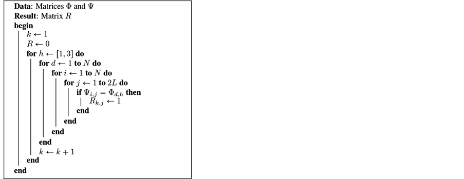
Algorithm 4. Generation of the matrix R.
2.3. Summary of the Method
We summarize this Section by declaring that the grayvalues of the estimated column can be solved from the Equation
 (1.21)
such that
![]() (1.22)
(1.22)
which can be easily gained by combining Equations (1.18) and (1.20).
Since the  cannot be uniquely defined from the Equation 1.22, the problem is ill-posed and it calls for regularization. The Tikhonov regularization algorithm was chosen, since it controls simultaneously residual
 ![]() and the norm of the solution
and the norm of the solution  (see chapter 2.3 in Kaipio and Somersalo (2005) for further information [41]). The Tikhonov solution for the Equation 1.22 has a form of
 (1.23)
where  is the regularization factor and
  is an identity matrix. The regularization factor can be based on the fact that in the non-local tomography the sum of each sinogram column is constant for throughout the sinogram. Therefore, the relaxation value
  can be calculated from the Equation
 (1.24)
The complete Algorithm 5 for defining  is described in details.
To calculate The Equation 1.23 less memory consuming, the Singular Value Decomposition (SVD) can be implemented for the matrix ![]() such that
such that . Then the Equation 1.23 has a matrix-free representation
 (1.25)
where  is the minimum dimension of the matrix
 . See for example Theorem 2.5 in Kaipio and Somersalo (2005) for proof [41].
So far we have described how to interpolate a single sinogram column. To interpolate all sinogram columns the procedure described in Sections from 2.2 to 2.2 are repeated for each unknown column. To numerically compute that, two nested loops are applied; an inner loop where the neighbor columns are fixed and the location of the estimated sinogram column varies and an outer loop where we change the neighbor columns. Before starting the actual interpolation process, we have to define how many new sinogram columns are needed for the isotropic resolution. If we generate too few new sinogram columns, we do not gain isotropic resolution. On the
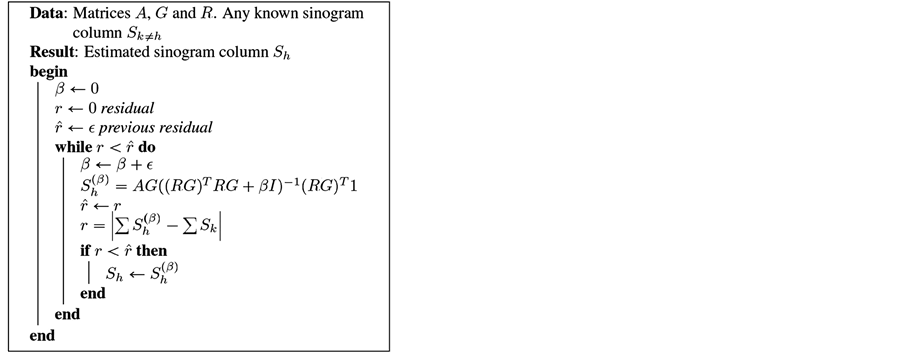
Algorithm 5. Generation of the Sinogram column Sh. Constant e is a small true positive number. See also Equation (1.25) for alternative way to calculate .
.
other hand, too many new sinogram columns just increases the computational burden without any improvements to the final reconstruction quality.
From Figure 1(c) we can see that
 (1.26)
where ![]() is the angular difference of the projection images,
is the angular difference of the projection images,  is the distance between two frequency components, and
 ![]() is the number of frequency samples. For simplicity,
is the number of frequency samples. For simplicity, ![]() is assumed to be odd and
is assumed to be odd and ![]() is constant.
is constant.
Based on the Fourier Slice Theorem, to gain uniform resolution in the frequency domain, the distance between frequency components within measurement  should be equal to the maximum distance between adjacent frequency components
  as discussed by Kak and Slaney (2001) and more deeply by Natterer (1986) [11,42]. Therefore, by defining
 , we can define Equation for optimal angular difference
  based on the Equation (1.26) as
 (1.27)
We introduce an interpolation factor ![]() such that
such that  where
where  is the original angular difference in sinogram. Then from the Equation (1.27) we get
 (1.28)
where  is the upward rounding operator.
The angle  for interpolated column
  can therefore be calculated from the Equation
 (1.29)
where . The detailed procedure for whole sinogram interpolation is described in the Algorithm 6.
3. Results
We used the GNU Octave program (version 3.2.3) with the imaging toolbox for numerical implementation of
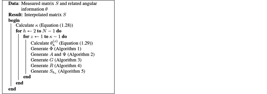
Algorithm 6. The SINT algorithm.
the SINT algorithm. The coding and executing environment was Ubuntu distribution version 10.04 including GNU/Linux operating system 2.6.32 and GNOME interface version 2.30.2. The computer that we employed for this study was a commercial 2.4 GHz dual-processor desktop computer with 8 GB of memory.
For the numerical implementation we adopted three synthetic phantoms with a size of ![]() pixels; Shepp-Logan, Dental Arc and Boxes. The standard Shepp-Logan phantom was chosen since it is widely used for evaluating the reconstruction image quality. The Dental Arc was calculated from full CT reconstruction of an artificial head (i.e. real teeth and skull embedded in an acrylic head) and therefore it can be considered as a reference for the clinical capability of SINT. Thirdly, the Boxes phantom consists of two isolated homogeneous rectangles to demonstrate a simplest possible case.
pixels; Shepp-Logan, Dental Arc and Boxes. The standard Shepp-Logan phantom was chosen since it is widely used for evaluating the reconstruction image quality. The Dental Arc was calculated from full CT reconstruction of an artificial head (i.e. real teeth and skull embedded in an acrylic head) and therefore it can be considered as a reference for the clinical capability of SINT. Thirdly, the Boxes phantom consists of two isolated homogeneous rectangles to demonstrate a simplest possible case.
Furthermore, these three phantoms were chosen to evaluate the capability of SINT because these phantoms generate essentially different kinds of sinogram representations, as shown in Figure 6. Since the Shepp-Logan phantom is a relatively isotropic object, it produces a smoothly varying sinogram. Secondly, the Dental Arc is a strongly anisotropic object, which produces a narrowing and widening sinogram with significant dynamic range in grayvalues. Finally, the Boxes phantom consists of two separate objects generating a branching and merging sinogram.
In all cases, we took nine synthetic projection images from ![]() to
to ![]() degree angles by using the built-in radon function. This function calculates the sum of pixels along a line with the given angles. The interpolation factor was set to
degree angles by using the built-in radon function. This function calculates the sum of pixels along a line with the given angles. The interpolation factor was set to ![]() based on Equation (1.28), which gave about
based on Equation (1.28), which gave about ![]() degrees angular differentiation for the final interpolated sinogram. We also evaluated the robustness of this method against pixel noise by adding Gaussian noise with variation of
degrees angular differentiation for the final interpolated sinogram. We also evaluated the robustness of this method against pixel noise by adding Gaussian noise with variation of ![]() of the pixel grayvalue to each known sinogram element.
of the pixel grayvalue to each known sinogram element.
As reference interpolation methods, we used linear, cubic spline and nearest neighbor -interpolation methods, which are the most common interpolation methods. For further information about these interpolation methods, see Section 4.4 in the book by the Gonzalez and Woods (2008) [30].
As an interpolation quality metric, we calculated relative ![]() norms against the ground truth. That is
norms against the ground truth. That is
 (1.30)
where  is the interpolated sinogram and
  is the noiseless sinogram generated from the original phantoms with similar angular difference than the interpolated sinograms. The results are shown in the Table2
We also reconstructed the object from the interpolated data for subjective comparison of reconstruction image quality. The reconstruction was executed by the built-in iradon -function, which executes Filtered BackProjection (FBP) reconstruction with a Ram-Lak -filter. The FBP was chosen since since it exposes the artifacts caused by interpolation flaws better than iterative methods like Algebraic Reconstruction Technique (ART), which have been considered as more suitable algorithms for the ill-posed situations (see for example Kolehmainen et al. (2003) or Siltanen et al. (2003)) [6,5]. For post-processing only linear grayvalue mapping was used to guarantee fair comparison. The authors prefer Kak and Slaney (2001) and Natterer (1986) for further information about the reconstruction algorithms and Gonzalez and Woods (2008) for post-processing [11,12,42]. The reconstruction results can be seen in Figure 2.
Table 2. The relative ![]() -norm of error in noiseless case and 5% noise added to projection images. The error is calculated as in the Equation (1.30).
-norm of error in noiseless case and 5% noise added to projection images. The error is calculated as in the Equation (1.30).
 (a)
(a)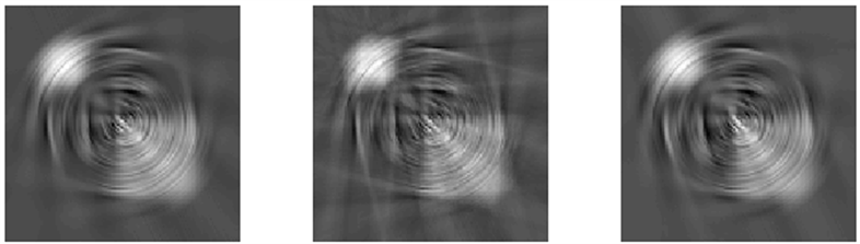 (b)
(b)
Figure 8. Profiles of the middle row in Shepp-Logan (top), Dental Arc (mid.) and Boxes (bottom) phantoms. The solid line is the profile of the original phantom, dashed is reconstruction with the SINT interpolation and dotted is the reconstruction with linear interpolation. Nearest neighbor and spline were not plotted because they produced very similar result than the linear interpolation.
4. Discussion
The results in this study are very preliminary. However, both qualitative and quantitative results suggest that SINT is significantly better than general interpolation routines when the angular data sampling is extremely sparse. This can be observed from the metrics as well as comparing the subjective image quality in Figures 2-4. See also the profiles in Figure 8.
In this study, we did not compare the SINT method against any sinogram-dedicated or state-of-the-art interpolation method for a number of reasons. Firstly, none of them are dedicated to as sparse a situation as our proposed method. For example, in the studies by Zhe et al. (2003) and Köstler et al. (2006) about ![]() of the sinogram columns were interpolated, while in our study over
of the sinogram columns were interpolated, while in our study over ![]() of the sinogram columns were interpolated [28,29]. Similarly, in the study by Penßel et al. (2005) only
of the sinogram columns were interpolated [28,29]. Similarly, in the study by Penßel et al. (2005) only ![]() of the sinogram columns were interpolated [30]. Secondly, part of the methods published recently are not fully documented or they require the right parameter settings for optimal result. Therefore, they cannot be used as reference since we could not guarantee a fair comparison. Thirdly, some of the new interpolation methods are designed for specific cases like the studies by Constantino (2006 and 2009) and earlier by Tam et al. (1990) [43-45]. These studies were limited to a situation where only the outer boundaries of isolated objects were modeled, while we concentrated on a more generic sinogram interpolation. Finally, we considered that a comparison with generally known interpolation algorithms gives a better understanding of the capability of this method than comparing to specific and dedicated interpolations.
of the sinogram columns were interpolated [30]. Secondly, part of the methods published recently are not fully documented or they require the right parameter settings for optimal result. Therefore, they cannot be used as reference since we could not guarantee a fair comparison. Thirdly, some of the new interpolation methods are designed for specific cases like the studies by Constantino (2006 and 2009) and earlier by Tam et al. (1990) [43-45]. These studies were limited to a situation where only the outer boundaries of isolated objects were modeled, while we concentrated on a more generic sinogram interpolation. Finally, we considered that a comparison with generally known interpolation algorithms gives a better understanding of the capability of this method than comparing to specific and dedicated interpolations.
There are two reasons why generic interpolation routines fail when they are applied to sparse sinograms. First, the generic interpolation methods do not take advantage of the characteristics of the sinogram. Second, the generic interpolation methods work only when there is a strong correlation between the neighbor sinogram values. However, when the distance from the known column increases the correlation between sinogram elements decreases. This vanishing correlation generates a whirlpool-shaped pattern which can be seen in the lower row of Figures 2-4. To verify these findings, we calculated the absolute error as a function of distance from the known sinogram column, i.e.:
 (1.31)
where ![]() is the distance from the known column to the interpolated column (with index
is the distance from the known column to the interpolated column (with index ![]() satisfying
satisfying , where
  is the interpolation factor as defined in Section 2.3). The influence of distance to the interpolation error can be seen in Figure 9, which shows that when the distance from the known sinogram column increases, the interpolation error of the SINT method increases significantly slower than the interpolation error of reference interpolation methods. The disadvantage of the SINT method is execution time, which in our examples was about
 ![]() s per interpolation. The most time consuming task was to verify that all warps intersect non-zero elements in the known columns as described in Section 2.2. Since every combination of the left and right neighbor column elements has to be considered as a warp candidate, the warp tracking operation has to be repeated
s per interpolation. The most time consuming task was to verify that all warps intersect non-zero elements in the known columns as described in Section 2.2. Since every combination of the left and right neighbor column elements has to be considered as a warp candidate, the warp tracking operation has to be repeated  times during the whole interpolation process, where
 ![]() is height of the sinogram,
is height of the sinogram,  is the number of original sinogram columns and
  is the interpolation factor. In this study, this meant over 4 million warp tracking operations. Another time consuming operation was the calculation of the eigenvalues for the matrix
![]() . In this study, we applied the Hessenberg and Schur decomposition based QR
. In this study, we applied the Hessenberg and Schur decomposition based QR
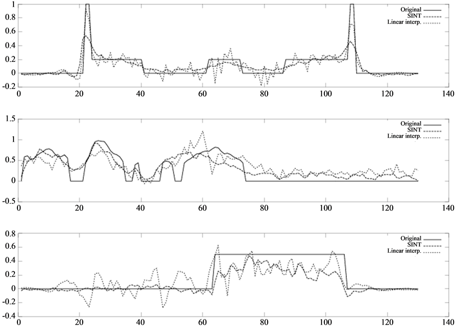
Figure 9. The SINT method (solid line), linear (long dash), spline (short dash) and nearest neighbor (dotted line) interpolation errors as a function of the distance from the known column for all three cases; Shepp-Logan (left), dental-arc (mid) and boxes (right). The error is calculated as described in the Equation (1.31).
algorithm, which is a well-known iterative method for defining the eigenvalues without the sorting procedure as discussed by Golub and Van Loan (1996) [39]. Since the matrix  was very sparse, positive-definite and orthogonal with only eigenvalues of one, the sorting procedure was irrelevant and only few iterations were needed.
There are number of articles indicating that parallel computing radically decreases the execution time in the image processing [46-48]. Despite the fact that we used a non-optimized high-level interpreted language in this study, the SINT method could easily be coded for a parallel processing environment, such as clustered computers or general purpose graphical processing unit (GP-GPU), by using OpenCL, Cuda or other parallel computing coding techniques. The parallelization of the SINT method is effective since the interpolated sinogram values are determined only from the original known sinogram columns, which are constant during the interpolation process and therefore they can be stored in fast read-only memory before executing the interpolation routine.
In this study, the SINT method has been proved to work in parallel beam imaging geometry cases in 2D, where the X-ray beam is perpendicular to the detector, instead of applying it to fan-beam in 2D or cone-beam in 3D. This limitation has been implemented partly for simplifying the theory and keeping the focus on the interpolation method itself. However, our interest is to expand this study to fan-beam and cone-beam imaging geometries in the near future. Our basic strategy for the parallel to fan beam conversion is based on modifying the warp matrix ![]() (see Section 2.2). As illustrated by Kak and Slaney (Chapters 3.4 and 3.5) [11], the projection angle in fan beam imaging geometry is the sum of the projection angle and the fan angle, i.e.:
(see Section 2.2). As illustrated by Kak and Slaney (Chapters 3.4 and 3.5) [11], the projection angle in fan beam imaging geometry is the sum of the projection angle and the fan angle, i.e.:
 (1.32)
where  is the fan angle, which depends on the sinogram element index. The fan angle can be calculated from the Equation
 (1.33)
where  is the shortest distance from X-ray source point to detector and
 ![]() is defined by Equation (1.12). This means that the angular value of each column
is defined by Equation (1.12). This means that the angular value of each column  is no longer constant, but depends on the row index of the sinogram element. Despite that this modification makes generation of the warp matrix
 ![]() more complex, the rest of the algorithm can be utilized per se. Finally, as shown by Kak and Slaney (Chapter 3.6), cone-beam geometry can be considered as a stack of fan beam sinograms and the 3D volume can be built by the interpolation process in the azimuthal direction.
more complex, the rest of the algorithm can be utilized per se. Finally, as shown by Kak and Slaney (Chapter 3.6), cone-beam geometry can be considered as a stack of fan beam sinograms and the 3D volume can be built by the interpolation process in the azimuthal direction.
5. Conclusion
Finally, very promising implication of the SINT method is in metal artifact reduction. Since metals are typically very radio-dense, they block a major part of the X-rays causing streak artifacts as indicated by Goldman and Fowlkes (2000) and Veldkamp et al. (2010) [49,50]. Since metallic areas can easily be seen in the sinogram as white regions, they can be identified, and the interpolation process could be used across these regions in the sinogram domain as indicated earlier by Ziying and Sze (1998), Yazdi and Beaulieu (2006), Meyer et al. (2009) or later by Abdoli et al. (2011) and Karimi et al. (2012) [15-18,51].
Acknowledgements
This research project was supported by the Instrumentarium Foundation and the Academy of Finland (project 141094 and the Finnish Centre of Excellence in Inverse Problems Research, decision number 250215). The authors wish to thank PaloDEx Group (Tuusula, Finland) and the Finnish Inverse Problems Society for their support. Finally, a special thanks to those who made this study possible by working on open source projects.
REFERENCES
- R. A. Brooks, G. H. Weiss and A. J. Talbert, “A New Approach to Interpolation in Computed Tomography,” Journal of Computed Assisted Tomography, Vol. 2, No. 5 1978, pp. 577-585.
- N. Hyvönen, M. Kalke, M. Lassas, H. Setälä and S. Siltanen, “Three-Dimensional X-Ray Imaging Using Hybrid Data Collected with a Digital Panoramic Device,” Inverse Problems and Imaging, Vol. 4, No. 2, 2010, pp. 257-271. http://dx.doi.org/10.3934/ipi.2010.4.257
- M. Rantala, S. Vänskä, S. Järvenpää, M. Kalke, M. Lassas, J. Moberg and S. Siltanen, “Wavelet-Based Reconstruction for Limited-Angle X-Ray Tomography,” IEEE Transactions on Medical Imaging, Vol. 25, No. 2, 2006, pp. 210-217. http://dx.doi.org/10.1109/TMI.2005.862206
- M. Varjonen, “Three-Dimensional Digital Breast Tomosynthesis in the Early Diagnosis and Detection of Breast Cancer,” Springer, Berlin, 2006.
- S. Siltanen, V. Kolehmainen, S. Järvenpää, J. P. Kaipio, P. Koistinen, M. Lassas, J. Pirttilä and E. Somersalo, “Statistical Inversion for X-Ray Tomography with Few Radiographs I: General Theory,” Physics in Medicine and Biology, Vol. 48, No. 10, 2003, pp. 1437-1463. http://dx.doi.org/10.1088/0031-9155/48/10/314
- V. Kolehmainen, S. Siltanen, S. Järvenpää, J. P. Kaipio, P. Koistinen, M. Lassas, J. Pirttilä and E. Somersalo, “Statistical Inversion for Medical X-Ray Tomography with Few Radiographs: II. Application to Dental Radiology,” Physics in Medicine and Biology, Vol. 48, No. 10, 2003, pp. 1465-1490. http://dx.doi.org/10.1088/0031-9155/48/10/315
- V. Kolehmainen, M. Lassas and S. Siltanen, “Limited Data X-Ray Tomography Using Nonlinear Evolution Equations,” SIAM Journal of Scientific Computing, Vol. 30, No. 3, 2008, pp. 1413-1429. http://dx.doi.org/10.1137/050622791
- R. L. Webber, R. A. Horton, D. A. Tyndall and J. B. Ludlow, “Tuned Aperture Computed Tomography, (TACT) Theory and Application for Three-Dimensional Dento-Alveolar Imaging,” Dentomaxillofacial Radiology, Vol. 26, No. 1, 1999, pp. 53-62. http://dx.doi.org/10.1038/sj.dmfr.4600201
- A. Cederlund, M. Kalke and U. Welander, “Volumetric Tomography—A New Tomographic Technique for Panoramic Units,” Dentomaxillofacial Radiology, Vol. 38, No. 2, 2009, pp. 104-111. http://dx.doi.org/10.1259/dmfr/16577933
- J. Hsieh, “Computed Tomography: Principles, Design, Artifacts, and Recent Advances,” SPIE Press, Bellingham, 2009.
- A. C. Kak and M. Slaney, “Principles of Computerized Tomography,” SIAM, 2001. http://dx.doi.org/10.1137/1.9780898719277
- R. C. Gonzalez and R. E. Woods, “Digital Image Processing,” 3rd Edition, Pearson Education Inc., Upper Saddle River 2008.
- P. La Riviere, “Noise Properties of Periodic Interpolation Methods with Implications for Few-View Tomography,” IEEE Transactions on Nuclear Science, Vol. 46, No. 3, 1999, pp. 639-645. http://dx.doi.org/10.1109/23.775592
- S. Schaller, T. Flohr, K. Klingenbeck, J. Krause, T. Fuchs and W. A. Kalender, “Spiral Interpolation Algorithm for Multislice Spiral CT. I. Theory,” IEEE Transactions on Medical Imaging, Vol. 19, No. 9, 2000, pp. 822-834. http://dx.doi.org/10.1109/42.887832
- Z. Y. Liu and F. Y. Sze, “A Sinogram Restoration Technique for the Hollow Projection Problem in Computer Tomography,” IEEE Proceedings of the 20th Annual International Conference of the Engineering in Medicine and Biology Society, Hong Kong, 29 October-1 November 1998, pp. 656-659.
- M. Yazdi and L. Beaulieu, “A Novel Approach for Reducing Metal Artifacts Due to Metallic Dental Implants,” IEEE Nuclear Science Symposium Conference Record, San Diego, 29 October-1 November 2006, pp. 2260-2263.
- E. Meyer, F. Bergner, R. Raupach, T. Flohr and M. Kachelriess, “Normalized Metal Artifact Reduction (NMAR) in Computed Tomography,” IEEE Nuclear Science Symposium Conference Record (NSS/MIC), Orlando, 24 October-1 November 2009, pp. 3251-3255.
- M. Abdoli, J. R. de Jong, J. Pruim, R. Dierckx and H. Zaidi, “Clough-Tocher Interpolation of Virtual Sinogram in a Delaunay Triangulated Grid Foal Artifact Reduction of PET/CT Images,” IEEE Nuclear Science Symposium and Medical Imaging Conference, Valencia, 23-29 October 2011, pp. 3197-3201.
- F. Sze and H. W. Y. Shum, “A Linear Sinogram Extrapolator for Limited Angle Tomography,” 3rd International Conference Signal Processing Beijing, 14-18 October 1996, pp. 386-389.
- D. R. Gilland, R. J. Jaszczak and R. E. Coleman, “Transmission CT Reconstruction for Offset Fan Beam Collimation,” IEEE Transactions on Nuclear Science, Vol. 47, No. 4, 2000, pp. 1602-1606. http://dx.doi.org/10.1109/23.873022
- L. Baojun and H. Jiang, “Comparison of Reconstruction Algorithms to Extend CT Reconstruction Field-of-View,” IEEE Nuclear Science Symposium Conference Record, 26 October-3 November 2007, pp. 3912-3914.
- A. A. Zamyatin and S. Nakanishi, “Sinogram Correction Methods Using Sinogram Decomposition,” IEEE Nuclear Science Symposium Conference Record, 29 October-1 November 2006, pp. 3438-3440.
- M. J. Lahart, “Estimation of Reconstructions in Computed Tomography,” Journal of Optical Society of America, Vol. 71, No. 10, 1981, pp. 1155-1161. http://dx.doi.org/10.1364/JOSA.71.001155
- C. R. Crawford and A. C. Kak, “Aliasing Artifacts in Computerized Tomography,” Applied Optics, Vol. 18, No. 21, 1979, pp. 3704-3711. http://dx.doi.org/10.1364/AO.18.003704
- T. Inouye, “Mage Reconstruction with Limited Angle Projection Data” IEEE Transactions in Nuclear Science, Vol. 21, 1979, pp. 2666-2669.
- D. L. Snyder and J. R. Cox, “An Overview of Reconstructive Tomography and Limitations Imposed by a Finite Number of Projections—Reconstruction Tomography in Diagnostic Radiography and Nuclear Medicine,” University Park Press, Baltimore, 1977.
- T. Sato, S. Norton, M. Linzer, O. Ikeda and M. Hirama, “Tomographic Image Reconstruction from Limited Projections Using Interactive Revision in Image and Transform Spaces,” Applied Optics, Vol. 20, No. 3, 1981, pp. 395-399. http://dx.doi.org/10.1364/AO.20.000395
- C. Zhe, B. Parker and D. Feng, “Temporal Compression for Dynamic Positron Emission Tomography via Principal Component Analysis in the Sinogram Domain,” IEEE Nuclear Science Symposium Conference Record, Vol. 4, 2003, pp. 2858-2862.
- H. Köstler, “Adaptive Variational Sinogram Interpolation of Sparsely Sampled CT Data” The 18th International Conference on Pattern Recognition, Hong Kong, Vol. 3, 2006, pp. 778-781.
- C. Penbel, M. Kachelrieb, M. Knaup and V. A. Kalender, “Azimuthal Interpolation and Noise Reduction,” IEEE Nuclear Science Symposium Conference Record, Vol. 4, 2005, pp. 1946-1949.
- M. Bertram, G. Rose, D. Schafer, J. Wiegert and T. Aach, “Directional Interpolation of Sparsely Sampled Cone-Beam CT Sinogram Data” Nano to Macro, International Symposium, Arlington, 15-18 April 2004, pp. 928-931.
- M. Bertram, J. Wiegert, D. Schafer, T. Aach and G. Rose, “Directional View Interpolation for Compensation of Sparse Angular Sampling in Cone-Beam CT,” IEEE Transactions on Medical Imaging, Vol. 28, No. 7, 2099, pp. 1011-1022. http://dx.doi.org/10.1109/TMI.2008.2011550
- A. Happonen, “Decomposition of Radon Projections into Stackgrams for Filtering, Extrapolation and Alignment of Sinogram Data,” Tampere University of Technology, 2005.
- J. Prince and A. Willsky, “Hierarchical Reconstruction Using Geometry and Sinogram Restoration,” IEEE Transactions on Image Processing, Vol. 2, No. 3, 1993, pp. 401-416. http://dx.doi.org/10.1109/83.236529
- R. W. Gerchberg, “Super-Resolution through Error Energy Reduction,” Optical Acta, Vol. 21, No. 9, 1974, pp. 709-720. http://dx.doi.org/10.1080/713818946
- A. Papoulis, “A New Algorithm in Spectral Analysis and Band-Limited Extrapolation,” IEEE Transactions in Circuits Systems, Vol. 22, 1975, pp. 735-742. http://dx.doi.org/10.1109/TCS.1975.1084118
- P. La Riviere, P. Xiaochuan and C-M. Kao, “Medical Imaging Applications of Effectively Multi-Dimensional Interpolation” Nuclear Science Symposium, Vol. 2, 1999, pp. 1023-1027.
- D. Bin, J. Lia and Z. Shen, “X-Ray CT Image Reconstruction via Wavelet Frame Based Regularization and Radon Domain Inpainting,” Journal of Scientific Computing, Vol. 54, No. 2-3, 2013, pp. 333-349. http://dx.doi.org/10.1007/s10915-012-9579-6
- G. Golub and C. F. Van Loan, “Matrix Computations,” 3rd Edition, The John Hopkins University Press, Baltimore, 1996.
- G. B. Arfken and H. J. Weber, “Mathematical Methods for Physicists,” Harcourt/Academic Press, San Diego, 2001.
- J. Kaipio and E. Somersalo, “Statistical and Computational Inverse Problems,” Springer-Verlag New York, 2005.
- F. Natterer, “The Mathematics of Computerized Tomography” John Wiley and Sons Ltd., Chichester; B. G. Teubner, Stuttgart, 1986.
- E. Constantino and K. Ozanyan, “Sinogram Enhancement for Tomographic Sensing Systems with Limited Resources,” IEEE Conference on Sensors, Daegu, 22-25 October 2006, pp. 514-517.
- E. Constantino and K. Ozanyan, “Tomographic Imaging of Surface Deformation from Scarce Measurements via Sinogram Recovery,” IEEE Sensors Journal, Vol. 9, No. 4, 2009, pp. 399-410. http://dx.doi.org/10.1109/JSEN.2008.2012195
- K. C. Tam, J. W. Eberhard and K. W. Mitchell, “Incomplete-Data CT Image Reconstructions in Industrial Applications,” IEEE Transactions on Nuclear Science, Vol. 37, No. 3, 1990, pp. 1490-1499. http://dx.doi.org/10.1109/23.57406
- S. Ha, S. Matej, M. Ispiryan and K. Müller, “GPU-Accelerated Forward and Backward Projection with Spatially Varying Kernels in 3D DIRECT TOF PET Reconstruction,” IEEE Transactions on Nuclear Science, Vol. 60, No. 1, 2013, pp. 166-173.
- K. S. Kyung and C. Y. Jong, “Fast Implementation of Fully Iterative Scatter Corrected OSEM for HRRT Using GPU,” IEEE Nuclear Science Symposium Conference Record (NSS/MIC), Knoxville, 30 October-6 November 2010, pp. 3330-3332.
- V. Kolehmainen, A. Vanne, S. Siltanen, S. Järvenpää, J. P. Kaipio, M. Lassas and M. Kalke, “Parallelized Bayesian Inversion for Three-Dimensional Dental X-Ray Imaging,” IEEE Transactions on Medical Imaging, Vol. 25, No. 2, 2006, pp. 218-228.
- L. Goldman and J. Fowlkes, “Categorical Course in diagnostic Radiology: CT and US Cross-Sectional Imaging,” RSNA, Oak Brook, 2000.
- J. H. Veldkamp, R. M. S. Joemai, A. J. van der Molen and J. Geleijns, “Development and Validation of Segmentation and Interpolation Techniques in Sinograms for Metal Artifact Suppression in CT,” Medical Physics, Vol. 37, No. 2, 2010, pp. 620-628. http://dx.doi.org/10.1118/1.3276777
NOTES

1This eigenvalue problem always has a solution based on the following fact: Since in each row and column in the matrix  there is exactly one non-zero component and for each non-zero element in
  holds
holds , the matrix
  is positively semi-definite and orthogonal and it has (only) eigenvalues of one.