Applied Mathematics
Vol.4 No.10C(2013), Article ID:38414,6 pages DOI:10.4236/am.2013.410A3011
Epidemic Propagation: An Automaton Model as the Continuous SIR Model
Mathematics Department, School of Science and Technology, University of Camerino, Camerino, Italy
Email: luciano.misici@unicam.it, filippo.santarelli@studenti.unicam.it
Copyright © 2013 Luciano Misici, Filippo Santarelli. This is an open access article distributed under the Creative Commons Attribution License, which permits unrestricted use, distribution, and reproduction in any medium, provided the original work is properly cited.
Received May 28, 2013; revised June 28, 2013; accepted July 5, 2013
Keywords: Cellular Automaton; SIR Model; Epidemic Spread
ABSTRACT
The use of the SIR model to predict the time evolution of an epidemic is very frequent and has spatial information about its propagation which may be very useful to contrast its spread. In this paper we take a particular cellular automaton model that well reproduces the time evolution of the disease given by the SIR model; setting the automaton is generally an annoying problem because we need to run a lot of simulations, compare them to the solution of the SIR model and, finally, decide the parameters to use. In order to make this procedure easier, we will show a fast method that, in input, requires the parameters of the SIR continuous model that we want to reproduce, whereas, in output, it yields the parameters to use in the cellular automaton model. The problem of computing the most suitable parameters for the reticular model is reduced to the problem of finding the roots of a polynomial Equation.
1. Introduction
Epidemics have always been a trouble for mankind and still continue to be: the globalization, since people can go from a side to the other of the Earth in a very fast way, can easily turn an infectious disease into a pandemic, perhaps spreading all over the world. Hence should be clear how helpful would be predicting when and where an epidemic will start and how it will evolve. Mathematical models, both deterministic and stochastic ones, which describe the evolution of population, can surely support this aim. SIR models, introduced for the first time in 1927 by Kermack and Mc Kendrick [1], are one of the most famous and used examples; they are a kind of models based on the partition of the population in three, or more classes, evolving over time according to a nonlinear ODE. The model can be complicated at will, adding the spatial distribution of the individuals, inserting an age structure or some stochastic terms to simulate the epidemics unpredictability [2-5].
As written above, further information about the spatial distribution can be achieved by adding partial derivatives terms right in the continuous SIR model, but we will not do that in this paper. Conversely, to pursue the same goal we will use a cellular automaton (CA), setting its parameters so that the disease evolution over time is similar to the one of the SIR models. This approach is very often used, but there is no way to know the best parameters to put in the reticular model unless you do a lot of tries and compare the results of several computations (see for example [6]). This calibration procedure is obviously quite imprecise and may lead to a very large waste of time.
In this paper we will describe a method to compute the CA model parameters on the basis of the ones of the continuous SIR models. Some assumptions must be made to use our method, but according to us they are not so strong and, when verified, the CA model perfectly simulates the results of the SIR model.
2. The SIR and SIRS Continuous Models and the Automaton Model
The models we are going to focus on are SIR and SIRS.
The first one takes its name from the division of the total population in three classes: susceptibles, those who can be infected during a contact with an ill individual, infectious, the ones who have contracted the disease but can recover, and recovered, individuals who cannot contract the disease again. The model consists of a system of non-linear ordinary differential Equations. Let ,
,  and
and  be the total number of susceptible, infectious and recovered individuals, respectively, at time
 ; suppose that the total number of individuals is constant over time and call it
 , so that
 .
.
The system of ODE that rules over our population is:
 (1)
(1)
with assigned initial conditions ,
,  and
and ;
;  is the density dependent parameter related to the average per capita contacts number and
  is the per capita recovery rate, that is the rate at which infected individuals recover; we have to suppose that
  is positive, otherwise it would mean that there is no cure for the disease.
SIRS model is ruled by the same system of non-linear ODE, except that a recovered individual can turn again into a susceptible one, situation that in some cases is related to the loss of immunity. We have to consider the new parameter , that is the rate at which recovered individuals change their state; we suppose
 , otherwise we would go back to the previous model. The system becomes:
 (2)
(2)
with the same initial conditions ,
, 
and .
.
In both of the previously described model we can add the class of vaccinated, evolving over time according to the function . Suppose we can only vaccinate susceptible individuals and we do that at the constant rate
  (if null we get the previous models), so that the systems (1) and become (with
  or
or  respectively):
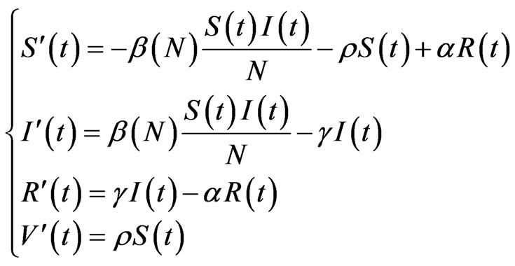 (3)
(3)
with the initial conditions ,
,  ,
,  and
and . Generally
  is quite big while
  is very small, because vaccination is mostly meant to be done before the disease spread, rather than once the epidemic has begun.
In this paper we will also consider a bidimensional probabilistic finite state cellular automaton in which we suppose that the individuals are static while the disease spreads. The cellular automaton model that we use is taken from [6]. In particular, supposing , we take an automaton made up of
  cells and
  total steps. At each step, we can represent it by a matrix
  made up of elements
  with
with ,
,  ,
, . At each step
 , each cell can assume exactly one of the possible states, whose number corresponds to the number of classes in the chosen model: in the following of this article we will assume
  if there is a susceptible at the
  -th row and the
  -th column,
  for an infectious,
  for a recovered and
  for a vaccinated. If we are at the step
 , the state transition for the cell at position
  is determined as following:
• Suppose . Let
. Let  be a matrix with elements
  representing the number of infectious in the Moore neighbourhood of radius
  of the current cell at the current step; we assume that the neighbourhood for each boundary cell is still the Moore one, except the cells that exceed the grid. Let
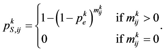
  be the probability matrix for susceptibles, where each element
  is the probability of the susceptible cell
  to become infectious in the
  -th step and it is given by
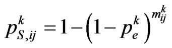 (4)
(4)
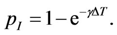
where  is the contagious probability at the current step. So generate a pseudo-random number
 , if
, if , then the current cell changes state and becomes infectious. In the Equation (4)
  is generally supposed to be constant over time, but we will not consider this condition from now on; the reason is that, with a constant
 , we haven’t a good simulation of the continuous model, while this was our aim.
If our continuous model contains the class  of vaccinated, we have to put it in the automaton; we introduce the probability
 , constant over time, that a susceptible becomes a vaccinated. Assume that vaccine has no effect on the individuals that have already contracted the disease, so that, if the current cell has changed its state, it cannot become vaccinated. If we still have
  instead, generate a new pseudo-random number
  and if
  then turn the current cell into a vaccinated.
• If , let
, let  be the probability that an infectious becomes recovered, then generate a new pseudo-random number
  and check if
 ; in this case the current cell becomes recovered.
• If  the cell is a recovered, so let
  be the probability that a recovered turns into a susceptible and generate a new pseudo-random number
 . If
. If  then the cell becomes a susceptible.
• In the case  the current cell cannot change its state, supposing vaccination never loses its effects.
3. As the Automaton Model Can Perfectly Simulate the Continuous SIR Model
Suppose we want to reproduce the behaviour of a SIR model with an automaton from the starting time  to the final time
 , so let
  be the time interval that corresponds to one step of our reticular model and
the number of steps that we require (we assume that  is such that
 ). We will see that we can arbitrarily set
  to get the best results, since it depends neither on the numerical method we choose to solve the continuous SIR model, nor on the step chosen for it.
Now focus on a single step of the automaton and put  with
with  and
and . Suppose we have to simulate from time
  to time
 . The structure of our automaton is such that a susceptible individual can only become infectious or vaccinated, while new susceptibles are generated only by the loss of immunity of recovered. So, if we want to calculate the probability that a susceptible becomes infectious, we have to focus on the decreasing of susceptibles due to the contact with infectious:
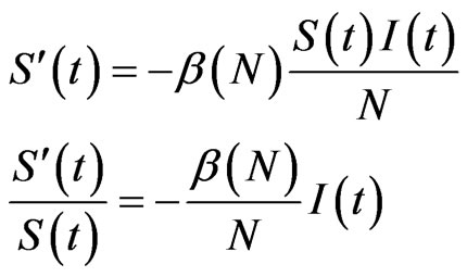
 (5)
(5)
Put 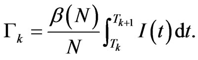 The integral
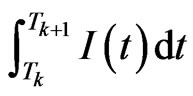
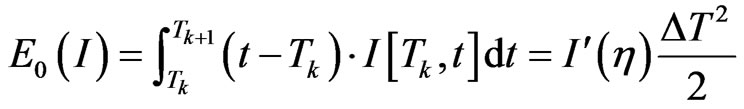
can be solved using a numerical method, for example we can approximate the function  using the interpolating polynomial of degree
  on the node
 , so:
, so:
Denoting  the first order divided difference, the integration error is estimated as follows:
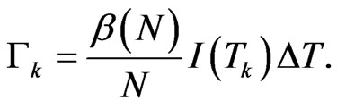
with . If we put
  we obtain
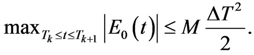 (6)
(6)
From Equation (5) we get
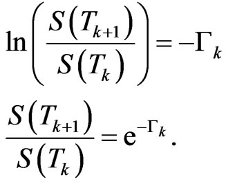
This is the fraction of susceptibles who are still healthy at  with respect to the initial value at
 ;
;  is the probability that a susceptible doesn't change its state, consequently
  is the probability that a susceptible becomes infectious.
Consider now the automaton model; put
 and
and  its cardinality, namely the total number of susceptibles at time
 . We are going to find the contagious probability
 , equal among all the individuals but changing step by step, so recall the transition probability for a susceptible:
For each susceptible we shall consider a stochastic variable , with
 , which assumes the value
  with a probability
 . The variable
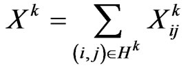
returns the number of susceptibles that change their status going from  to
to . If we put
 that is the set of susceptibles that are able to turn into infected, and
  its cardinality, we can calculate the expected value of
  as shown below:
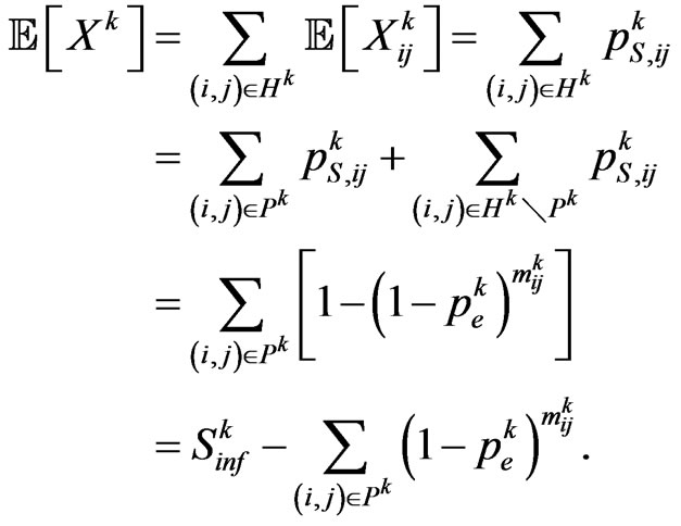
We expect that  individuals become infectious at this step. Since our aim is to reproduce the SIR model, we must make the automaton model not dependent on the spatial distribution of individuals at time
 , otherwise each computation would lead to different results. Hence we force
  to be equal to the number of susceptibles that change class in the continuous model, namely
 , so that we get:
 (7)
(7)
Equation (7) is just what we need: we only have to find its roots, if present, to get the most suitable value of  to reproduce the SIR model. In the following we will show that the function
  defined as
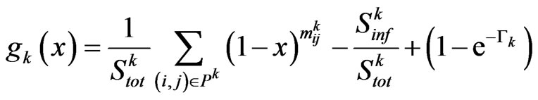
under a particular condition admits exactly one zero in the interval .
.
We can see that  as combination of continuous functions and
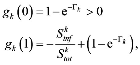
therefore there exists at least one zero of  in
in  if
if
 (8)
(8)
Furthermore we have
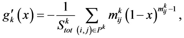
that is negative in all the open interval , hence the zero, if exists, is unique. So if
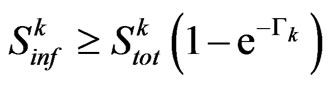 , Equation has exactly one root, that is the probability
  that we need.
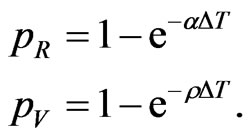
Finally we have to calculate the remaining parameters in order to use the automaton model. As in Equation (5), focusing on the decreasing of infectious we get

Now  is the probability that an infectious doesn’t change its state and consequently
 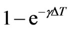 is the probability that he becomes recovered. Hence we have:
Similarly we can compute the other parameters:
We have found that the automaton could perfectly simulate a SIR model, if the condition (8) is satisfied: it states that the number of susceptibles able to be infected must be greater than (or equal to) the number of them who must change their state (according to the continuous model). If, at a certain step of the computation, we found that the relation (8) is no more verified, we can reasonably force  to the value
 , so that all the susceptibles able to become ill do it and the results of the automaton are as close to the ones of the continuous model as possible. If the computation with the automaton is not satisfying yet we can reduce
  until the condition (8) is verified at any step: indeed the number
  decreases since
  linearly depends on
 , whereas
  remains the same, because it depends just on the spatial distribution of infected individuals. We can also notice that the integration error given by Equation (6) consequently reduces.
4. Some Results
We will show in this section some results obtained with the automaton and compare them to the respective solution given by the continuous SIRS model.
For the simulation we took an automaton of  cells disposed in a
  grid; we have found that using more individuals doesn’t lead to good images in the printed version of the spatial distribution, so we decided to limit
  and improve the quality of the figures. We set the initial conditions to
 ,
,  ,
,  and the parameters of the SIRS model to
 ,
,  ,
,  and
and , with
  and
and . With the method proved above we computed the parameters for the automaton model, then we randomly generated the initial matrix
  and ran a simulation using
 . The computation led to Figure 1. At time
 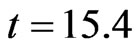 (that is at the step
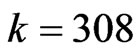 ) the infection reached its peak and the spatial distribution of the individuals is shown in Figure 2. Since we want to compare this simulation of the disease with a numerical solution of the SIRS model, we decided to use the Euler’s method with a step
 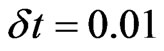 to solve the system (the solution is reported in Figure 3). We can notice that the two approaches give quite the same results; however our method yields the spatial distribution of the individuals and allows the use of a cellular automaton to simulate a disease spread: this means involving a discrete population and the unpredictability of an epidemic.
From Equation (6) we can notice that the approximation

Figure 1. Disease evolution over time according to the automaton model.

Figure 2. Spatial configuration of individuals at time t = 15.4.
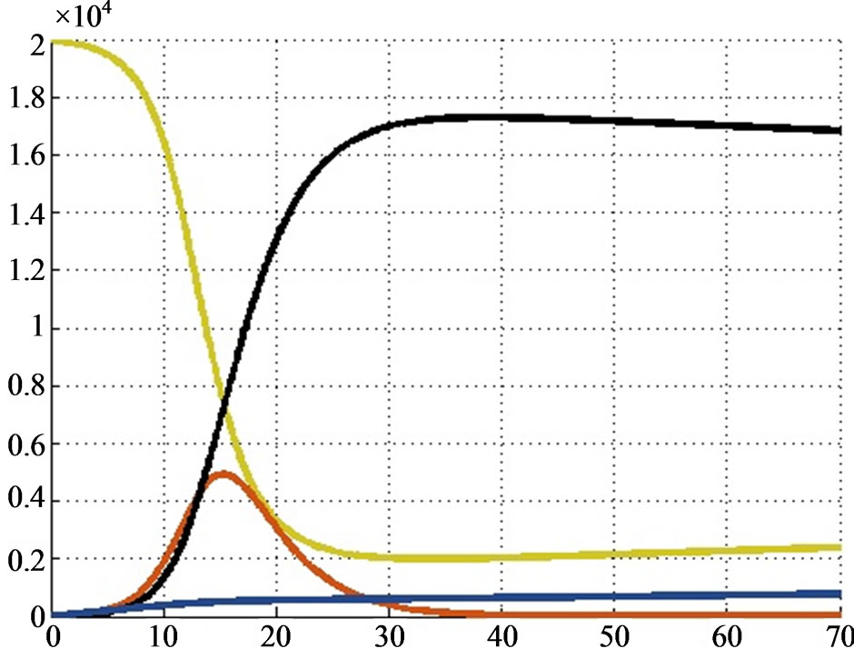
Figure 3. Numerical solution of the SIRS model given by Euler’s method.
error may increase if  increases in the interval
 ; hence we thought to test our algorithm also in this case. We have decided to change the following parameters:
 ,
,  and
and . Figure 4 shows the solution given by our algorithm, while Figure 5 shows Euler’s one. We can see that the two solutions
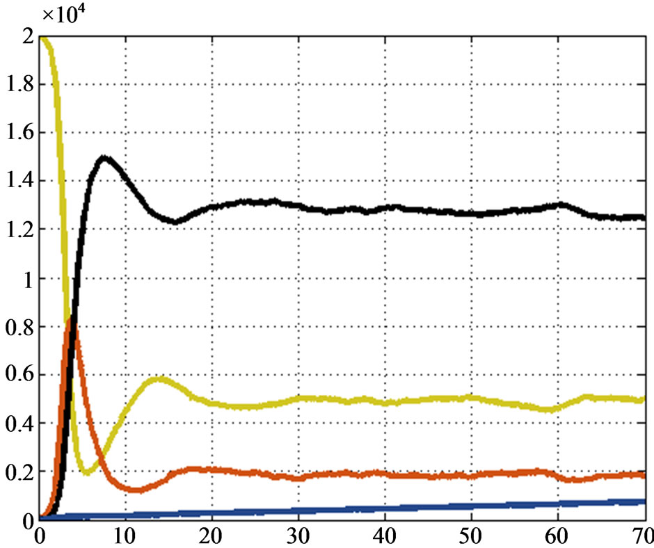
Figure 4. Second test: solution provided by the automaton model.
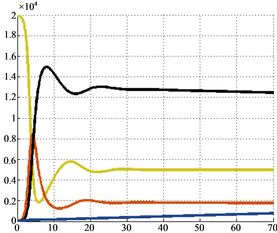
Figure 5. Second test: solution given by the Euler’s method.
are quite the same, so our method works also in the worst situations.
We tested our algorithm also over an automaton with  and, after 140 steps, the simulation finished in 222.29 seconds, so it is very fast. It can be probably adapted to solve also other systems of ODEs, for which a spatial evolution of the involved functions is useful, although the simulations in these cases may be not satisfying; that because we have chosen a particular cellular automaton, with its own law of transition and type of neighbourhood, which well describe the spread of an epidemic, but probably are not good in another framework. Our future work will be trying to generalize this method to other systems of ODEs (including more complicated epidemic models that better reproduce the behaviour of a real disease) and to other types of cellular automata.
REFERENCES
- W. O. Kermack and A. G. McKendrick, “A Contribution to the Mathematical Theory of Epidemics,” Proceedings of the Royal Society of London A, Vol. 115, No. 772, 1927, pp. 700-721. http://dx.doi.org/10.1098/rspa.1927.0118
- C. Castillo-Chavez, H. W. Hethcote, V. Andreasen, S. A. Levin and W. M. Liu, “Epidemiological Models with Age Structure, Proportionate Mixing, and Cross-Immunity,” Journal of Mathematical Biology, Vol. 27, No. 3, 1989, pp. 233-258. http://dx.doi.org/10.1007/BF00275810
- V. Capasso, “Mathematical Structures of Epidemic Systems,” Lecture Notes in Biomathematics, Vol. 97, 1993. http://dx.doi.org/10.1007/978-3-540-70514-7
- I. Nåsell, “Stochastic Models of Some Endemic Infections,” Mathematical Biosciences, Vol. 179, No. 1, 2002, pp. 1-19. http://dx.doi.org/10.1016/S0025-5564(02)00098-6
- N. T. J. Bailey, “The Simulation of Stochastic Epidemics in Two Dimensions,” Proceedings of the Fifth Berkeley Symposium on Mathematical Statistics and Probability, University of California Press, Berkeley, Vol. 4, 1967, pp. 237-257.
- S. Chang, “Cellular Automata Model for Epidemics,” 2008. http://csc.ucdavis.edu/~chaos/courses/nlp/Projects2008/SharonChang/Report.pdf