Applied Mathematics
Vol.4 No.4(2013), Article ID:30444,5 pages DOI:10.4236/am.2013.44092
An Adaptive Least-Squares Mixed Finite Element Method for Fourth Order Parabolic Problems
Department of Mathematics, Qingdao University of Science and Technology, Qingdao, China
Email: *ghm@qust.edu.cn
Copyright © 2013 Ning Chen, Haiming Gu. This is an open access article distributed under the Creative Commons Attribution License, which permits unrestricted use, distribution, and reproduction in any medium, provided the original work is properly cited.
Received January 29, 2013; revised February 22, 2013; accepted March 1, 2013
Keywords: Adaptive Method; Least-Squares Mixed Finite Element Method; Fourth Order Parabolic Problems; Least-Squares Functional; A Posteriori Error
ABSTRACT
A least-squares mixed finite element (LSMFE) method for the numerical solution of fourth order parabolic problems analyzed and developed in this paper. The Ciarlet-Raviart mixed finite element space is used to approximate. The a posteriori error estimator which is needed in the adaptive refinement algorithm is proposed. The local evaluation of the least-squares functional serves as a posteriori error estimator. The posteriori errors are effectively estimated. The convergence of the adaptive least-squares mixed finite element method is proved.
1. Introduction
A general theory of the least-squares method has been developed by A. K. Aziz, R. B. Kellogg and A. B. Stephens in [1]. The most important advantage leads to a symmetric positive definite problem. In the least-squares mixed finite element approach, a least-squares residual minimization is introduced. This method has an advantage which is not subject to the LBB [1] condition. The mixed finite element methods of least-squares type have been the object of many studies recently (see, e.g. Stokes Equation [2], Elliptic Problem [3], Newtonian Fluid Flow Problem [4], Transmission Problems [5], Sobolev Equations [6], Parabolic Problems [7] et al.). The adaptive least-squares mixed finite element method have been studied in recent several years (see, e.g. the linear elasticity [8]), but the research of adaptive method about fourth order parabolic problems is not common.
Adaptive methods are now widely used in the scientific computation. In this paper, we are interested in the adaptive least-squares mixed finite element method for fourth order parabolic problems, fourth order parabolic problems are fundamental partial differential equations. It occurs in various areas of applied mathematics and science. Our emphasis in this paper is on the performance of an adaptive refinement strategy based on the a posteriori error estimator inherent in the least-squares formulation by the local evaluation of the functional. During the last 15 - 20 years a big amount of work has been devoted to a posteriori error estimation problem, i.e., computing reliable bounds on the error of given numerical approximation to the solution of partial differential equations using only numerical solution and the given data. In order to operate the a posteriori error estimator should be neither under nor overestimate the error. The a posteriori error is effectively estimated, and proved the convergence of the adaptive least-squares mixed finite element method in this paper.
An outline of the paper is as follows. The least-squares formulation of fourth order parabolic problems is described in Section 2. It includes continuous and coercivity properties of the least-squares variational formulation. Appropriate spaces for the finite element approximation and a generalization of the coercivity shown in Section 2 to the discrete form is discussed in Section 3. In Section 4, a posteriori error estimators which are needed in an adaptive refinement algorithm are composed with the least-squares functional, and posteriori errors are effectively estimated. The convergence of the adaptive leastsquares mixed finite element method is shown in Section 5. Finally, we summarize our findings and present conclusions in Section 6. In this paper, we define C to be a generic positive constant.
2. A Least-Squares Formulation of Fourth Order Parabolic Problems
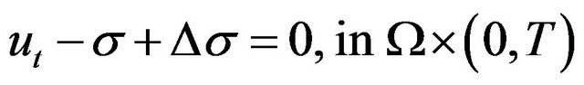
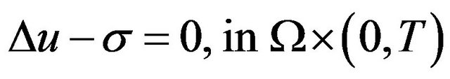
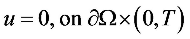
We start from the equations of fourth order parabolic problems in the form:
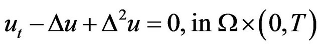 (1)
(1)
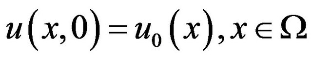
 (2)
(2)
 (3)
(3)
 (4)
(4)
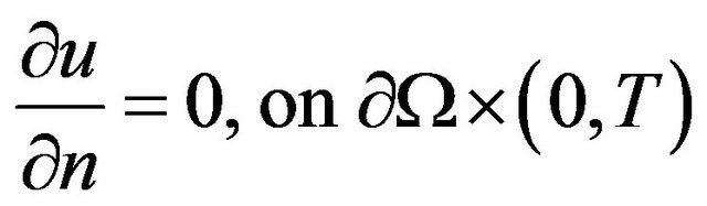
where 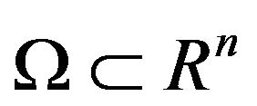 is a bounded domain, with boundary
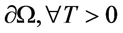 . We shall consider an adaptive least-squares mixed finite element method for (1)-(4).
Now we set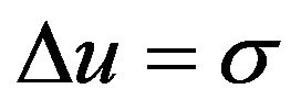 , then, we have:
 (5)
(5)
 (6)
(6)
 (7)
(7)
 (8)
(8)
 (9)
(9)
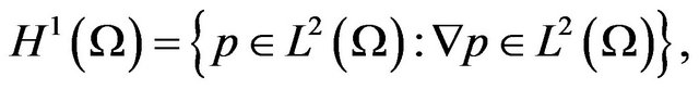
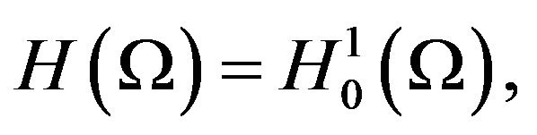
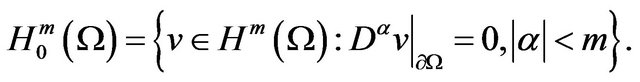
We introduce the Sobolev spaces:
Now, let us define the least-squares problem: find 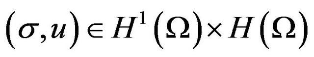 [9] such that
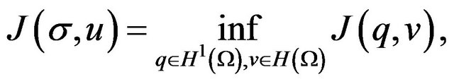 (10)
(10)
where
 (11)
(11)
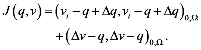
We introduce the least-squares functional:
![]()
Taking variations in (10) with respect to q and v, the weak statement becomes: find  such that
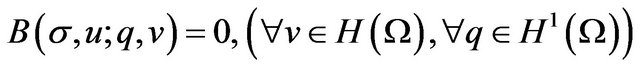 (12)
(12)
where
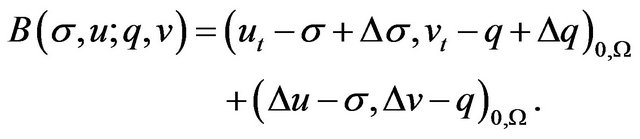 (13)
(13)
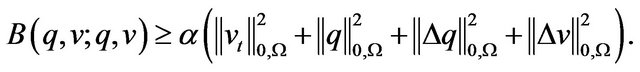
Theorem 2.1. The bilinear form  is continuous and coercive. In other words, there exist positive constants
 ![]() and
and , such that

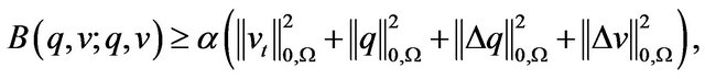
holds for all .
.
Proof: 1) For the upper bound we have:
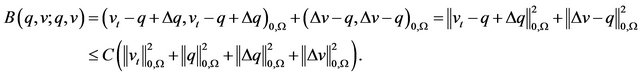
Since the bilinear form is symmetric, this is sufficient for the upper bound in Theorem 2.1.
2) For the lower bound.
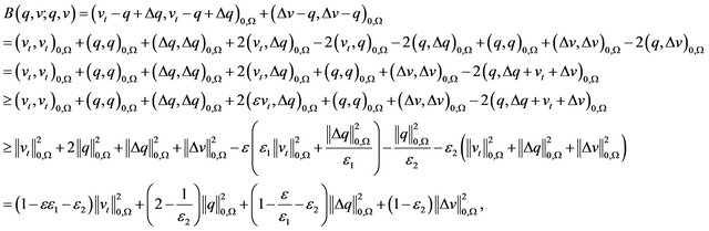
so we can select the positive constants  satisfying
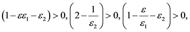
we have
The proof of Theorem 2.1 is therefore completed.
Theorem 2.2. The Equations (5)-(9) has a unique solution, and the solution is .
.
Proof: From Theorem 2.1, we know that the bilinear form  is coercive and bounded on
 . Then the result follows from Lax-Milgram theorem.
3. Finite Element Approximation
In principle, the LSMFE approach simply consists of minimizing (12) in finite-dimensional subspaces 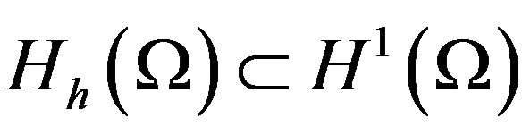 and
and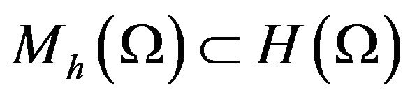 . Suitable spaces are based on a triangulation
  of
of  and consist of piecewise polynomials with sufficient continuity conditions.
Now we consider the Ciarlet-Raviart mixed finite element form. Let 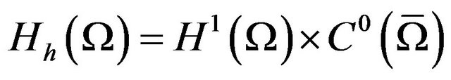 and
and
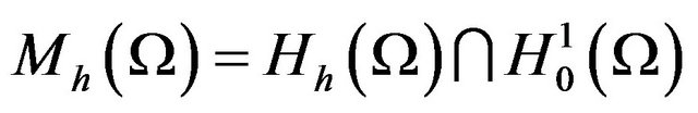 , let
, let  be a class qusi-uniform regular partition of
 .
.
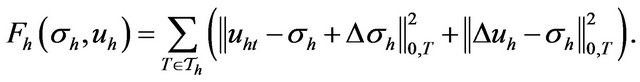
The least-squares functional:
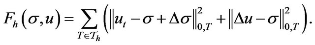 (14)
(14)
Minimizing the functional (14) is equivalent to the following variational problem: find  and
and  such that
 holds for all
 .
.
The discrete bilinear form  is defined as follows:

which holds for all 
 .
.
Theorem 3.1. The bilinear  is continuous and coercive, i.e., there exist positive constants
  and
and  such that

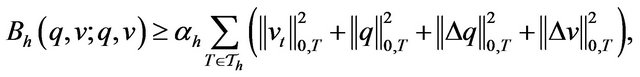
which holds for all 
 . The proof is the same as the Theorem 2.1, we omit the proof.
4. Postieriori Error Estimation
One of the main motivations for using least-squares finite element approaches is the fact that the element-wise evaluation of the functional serves as an a posteriori error estimator.
A posteriori estimate attempt to provide quantitatively accurate measures of the discretization error through the socalled a posteriori error estimators which are derived by using the information obtained during the solution process. In recent years, the use of a posteriori error estimators has become an efficient tool for assessing and controlling computational errors in adaptive computations [10].
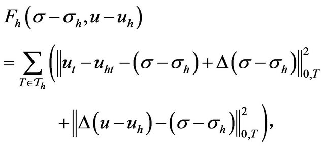
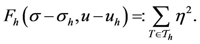
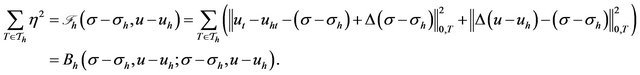
Now we define the least-squares functional:
 (15)
(15)
We have
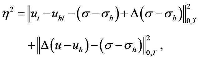
so we define the posteriori estimator as following:
 (16)
(16)
Theorem 4.1. The least-squares functional constitutes an a posteriori error estimator. In other words, for
there exist positive constants  and
and  such that


Proof: We know
From Theorem 3.1, we have:


The positive constants  and
and , this completes the proof.
Remark: The mesh is adapted and based on a posteriori error estimate of the fourth order elliptic problems. Based on the computed a posteriori error estimator , we use a mesh optimization procedure to compute the size of elements in the new mesh. Adaptive refinement strategies consist in refining those triangles with the largest values of
 .
.
5. Convergence Analysis of Adaptive Least-Squares Mixed Finite Element Method
We now briefly introduce the main idea of adaptive leastsquares mixed finite element methods through local refinement. Given an initial triangulation , we shall generate a sequence of nested conforming triangulations
  using the following loop
 :
:

More precisely to get  from
from  we first solve (5)-(9) to get
  on
on . The error is estimated using
  and to mark a set of
  that are to be refined. Triangles are refined in such a way that the triangulation is still shape regular and conforming.
The a posteriori error estimator is essential part of the ESTIMATE step. The a posteriori error estimator is usually split into local error indicators and they are then employed to make local modifications by dividing the elements whose error indicator is large and possibly coarsening the elements whose error indicator is small.
The convergence of local refinement algorithms based on the repetition of loop  is established by the error reduction type result. Let
  be a shape regular triangulation of
  and
and  is a refinement of
  such that
 . Let
. Let  and
and  be the finite element approximation of
 ![]() in
in  and
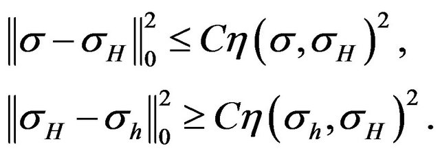
and , respectively. We shall use the following results in the proof of the convergence [11]:
![]() (17)
(17)
Let  be an initial shape regular triangulation, let
  be a solution of (5)-(9) in the
 ![]() loop. We have the following theorem:
loop. We have the following theorem:
Theorem 5.1. Let  be a solution obtained in the
 ![]() loop in the algorithm, then there exists a constants
loop in the algorithm, then there exists a constants  depending the shape regularity of
  such that:
![]()
and thus the algorithm will terminate in finite steps.
Proof: In the  step we select
  such that
From Theorem 4.1, we obtain the following inequality:
By (17) we have:
![]()
so there exists a constant  such that
![]()
we let![]() , we then get
, we then get
which by recursion implies
So the adaptive least-squares mixed finite element method is converged.
6. Summary and Conclusions
We describe an adaptive least-squares mixed finite element procedure for solving the fourth order parabolic problems in this paper, and the procedure uses a leastsquares mixed finite element formulation and adaptive refinement based on a posteriori error estimate. The methods were applied to study the continuous and coercivity of the fourth order parabolic problems.
In this paper, we applied relatively standard a posteriori error estimation techniques to adaptively solve the fourth order parabolic problems and shown the convergence of the adaptive least-squares mixed finite element method.
REFERENCES
- A. K. Aziz, R. B. Kellogg and A. B. Stephens, “LeastSquares Methods for Elliptic Systems,” Mathematics of Computation, Vol. 44, 1985, pp. 53-70. doi:10.1090/S0025-5718-1985-0771030-5
- H. M. Gu, D. P. Yang, S. L. Sui and X. M. Liu, “LeastSquares Mixed Finite Element Method for a Class of Stokes Equation,” Applied Mathematics and Mechanics, Vol. 21, No. 5, 2000, pp. 557-566. doi:10.1007/BF02459037
- H.-M. Gu and X.-L. Xu, “The Least-Squares Mixed Finite Element Methods for a Degenerate Elliptic Problem,” Mathematica Applicata, Vol. 15, No. 1, 2002, pp. 118- 122.
- Z. Q. Cai, B. Lee and P. Wang, “Least-Squares Methods for Incompressible Newtonian Fluid Flow: Linear Stationary Problems,” SIAM Journal on Numerical Analysis, Vol. 42, No. 2, 2004, pp. 843-859. doi:10.1137/S0036142903422673
- M. Maischak and E. P. Stephan, “A Least Squares Coupling Method with Finite Elements and Boundary Elements for Transmission Problems,” Computers & Mathematics with Applications, Vol. 48, No. 7-8, 2004, pp. 995-1016. doi:10.1016/j.camwa.2004.10.002
- H. M. Gu and D. P. Yang, “Least-Squares Mixed Finite Element Method for Sobolev Equations,” Indian Journal of Pure and Applied Mathematics, Vol. 31, No. 5, 2000, pp. 505-517.
- M.-Y. Kim E.-J. Park and J. Park, “Mixed Finite Element Domain Decomposition for Nonlinear Parabolic Problems,” Computers & Mathematics with Applications, Vol. 40, No. 8-9, 2000, pp. 1061-1070. doi:10.1016/S0898-1221(00)85016-6
- Z. Q. Cai, J. Korsawe and G. Starke, “An Adaptive Least Squares Mixed Finite Element Method for the StressDisplacement Formulation of Linear Elasticity,” Numerical Methods for Partial Differential Equations, Vol. 21, No. 1, 2005, pp. 132-148. doi:10.1002/num.20029
- Z. D. Luo, “Theoretical Bases for Mixed Finite Element Methods and Application,” Science Press, Beijing, 2006.
- S.-Y. Yang, “Analysis of a Least Squares Finite Element Method for the Circular Arch Problem,” Applied Mathematics and Computation, Vol. 114, No. 2-3, 2000, pp. 263-278. doi:10.1016/S0096-3003(99)00122-8
- T. Tang and J. C. Xu, “Adaptive Computations: Theory and Algorithms,” Science Press, Beijing, 2007.
- A. Agouzal, “A Posteriori Error Estimators for Nonconforming Approximation,” Mathematical Modelling and Numerical Analysis, Vol. 5, No. 1, 2008, pp. 77-85.
- X. Li, M. S. Shephard and M. W. Beall, “3D Anisotropic Mesh Adaptation Using Mesh Modifications,” Submitted to Computer Methods in Applied Mechanics and Engineering, 2003.
NOTES
*Corresponding author.