Applied Mathematics
Vol. 3 No. 12A (2012) , Article ID: 26014 , 9 pages DOI:10.4236/am.2012.312A287
The Markovian Approach for Probabilistic Life-Cycle Assessment of Existing Structures
Department of Structural Engineering, Politecnico di Milano, Milano, Italy
Email: elsa.garavaglia@polimi.it
Received August 28, 2012; revised November 12, 2012; accepted November 19, 2012
Keywords: Structural Deterioration Process; Transition Processes; Markov Renewal Processes; Lifetime Assessment; Selective Maintenance Planning
ABSTRACT
The reliability of structural systems, lying in aggressive environments, changes over time. Proper maintenance is usually required to achieve a suitable performance level of life-cycle. The damage process affecting the systems often suffers from uncertainty due to the randomness involved in each environmental attack. Therefore, basing on suitable damage modeling as well as on probabilistic analysis, the main features of time-variant deterioration process are modeled and then the life-cycle is assessed. On the basis of Markov renewal theory (MRT), this paper proposes a combined approach using an appropriate time dependent damage model and probabilistic analysis. Since repairing deteriorated structures requires the arrangement of maintenance strategies, possible selective maintenance scenarios have to be considered. Referring to the relationship between MRT and an appropriate condition index, some repair strategies have been proposed and compared with each other. Those strategies are applied just to seriously deteriorated members. Furthermore selective maintenance benefits are economically investigated.
1. Introduction
Since any structural system in aggressive environment suffers from deterioration over time, the damage increases, while some structural capabilities decreases [1, 2]. Thence system’s performance is reduced. Usually deterioration laws governing environmental aggression are unknown; therefore, just a stochastic approach enables to assess the life-cycle of the system [3,4].
Biondini and Garavaglia [5] refer to the life-cycle of a deteriorated structure as a reliability problem, where a loss of performance greater than a prescribed threshold value is considered as a failure. When a failure occurs, the system moves from the current state to another one characterized by a lower level of performance. Maintaining and/or repairing lead to the opposite process: the system moves from an initial low state of performance to a higher one. Both cases describe the failure process as a transition process through different states, due to environmental attacks and/or maintenance actions.
Assuming the Markov Renewal Process (MRP) as the most suitable stochastic dynamic method, the transition process can be modelled [6,7].
MRP is usefully applied in predicting natural hazard and catastrophic events (e.g. earthquakes and typhoons) [7-13] as well as in forecasting material deterioration over time [14-17]. Thence MRP seems to be the best approach for modelling the deterioration of structures in aggressive environment.
Basing on MRP, a deteriorated steel truss has been chosen as the case study for assessing life cycle reliability and planning selective maintenance strategies. Material damage is described in probabilistic terms within a Markov renewal model [14]. The probability of the system’s transition through different performance states has been investigated. Regarding results from Markov method, some selective maintenance scenarios have been discussed. Repair interventions have just been applied to seriously deteriorated members and/or characterized by a low safety margin. Thence following Biondini et al. [7] approach, a suitable condition index is used. Considering the effects of selective maintenance, the here proposed procedure has been applied to life-cycle reliability analysis and maintenance planning of a steel truss structure [18].
2. Markov Renewal Processes and Structural Deterioration Processes
The deterioration process can be seen as a loss of performance affecting a material system. Whenever deterioration reaches a given threshold, the system suffers a “failure” and a loss of performance. This phenomenon can be described as the transition of the system (i.e. the material) through different service states characterized by different levels of performance. Thus, the deterioration process (failure process) may be defined as a transition process [14].
Every transition depends on:
• Magnitude of attack (stress cycle).
• System’s capability to withstand the attack.
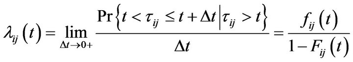
Both these parameters depend on a large number of time dependent random variables (r.v.); therefore the transition process is rightly interpreted as a stochastic process. A possible r.v. which can be assumed to describe a transition process is the service lifetime ti defined as “the waiting time spent by the material in the performance state i before a transition” [14].
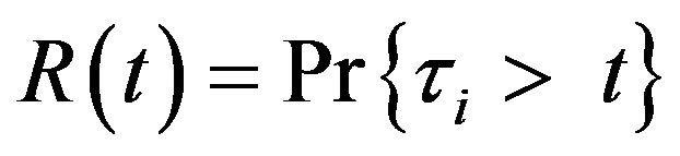
From this point of view the reliability function  can be defined as:
 . (1)
. (1)
Equation (1) is the probability that a transition from state i to a next state doesn’t happen by waiting time ti [19], and it can be described as the survival function of the r.v. ti.
If the deterioration process is assumed to be a transition process, a stochastic dynamic process can be assumed to represent it, and Biondini and Garavaglia [5] have shown that the Markov Renewal Process (MRP) seems to be suitable method to describe it [6,7]. MRP are a class of stochastic processes generalizing the Markov jump process as well as the renewal process. It can illustrate the evolution of the system’s life through different service states with different waiting times, and it also enables to consider the age t0 of the system, i.e. the time already spent by the system in the current service state before the prediction is made. This aspect is very important in reliability analysis when maintenance must be planned.
2.1. Introducing Markov Renewal Processes
Here has been proposed a brief review of both the definition and some properties of the MRP with a finite state space where, for  with
with 
 denotes a matrix of the distribution functions on
 ,
, 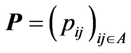 denotes a transition matrix on A, and
 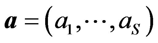 a probability distribution on A
(i.e.  and
and ).
).
Considering a two-dimensional stochastic process
 defined in a complete probability space
 satisfying [6,7]:
1) Initial conditions of t0 = 0 a.s.
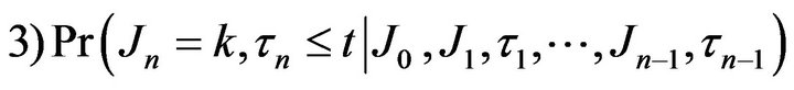
2)  for every k Î A.
 a.s. for every
  and
and .
.
The probabilities  are the transition probabilities of the Markov chain
  and
and  are the distribution functions associated to waiting times in the state Jn−1 before moving to the next state
 .
.
DEF. The process  is called the MRP and is determined by
 .
.
Some consequences of that definition are recalled hereunder:
1)  is a A-valued Markov chain with transition matrix P and initial distribution a.
2) for every n>1, τ1, ,τn are conditionally independent, given
  and
and
 a.s. (2)
The Markov chain  represents the states successively visited, and the process
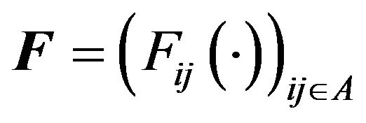
  represents the successive waiting times. The application here proposed assumes the performance levels reached by a structural system along its life as the transitory states. Those levels have been classified with respect to different damage severity. τn are the waiting times between successive losses of performance. Basing on 2) consequence, if damage is classified by severity i Î A and the next damage severity is j Î A, the time between the two losses of performance is a positive random variable with distribution Fij, and density fij, for every i, j = 1,
  , S.
, S.
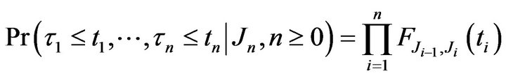
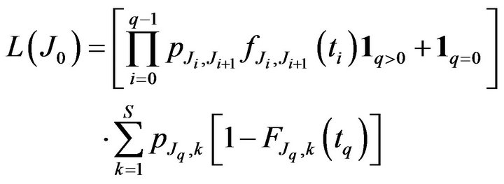
Supposing (J0, J1, t1, ..., tq−1, Jq) describes the MRP within the time-window [0,T], q represents the number of states visited over [0,T]. Thence the last event Jq has an incomplete waiting time tq, which represents the censored data: 
Thus, the conditional likelihood is:
 (3)
(3)
where  and
and 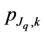 are the transition probabilities defined above,
 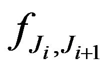 and
and 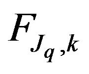 are the density and the cumulative distribution of the probability distribution function chosen and 1 stands for indicator functions.
Maximizing the log-likelihood over the time-window , the maximum likelihood for
  and for the parameters of
  has been estimated.
2.2. Crossing State Prediction
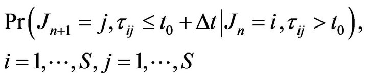
Knowing the last transition state i as well as the time t0 passed since the transition occurred, the j-state of next transition in a lower performance level has been predicted.
When the MRP is defined (points I-III), considering t0 as the time already passed by the system in the current i-state, the probability that the system will pass to state j is:
 (4)
(4)
Jn is the state of the present performance, Jn+1 is the state of next reduced performance, τij is the waiting time spent by the system in the state i before moving on j, under the condition that no transition has already occurred (defined by the condition: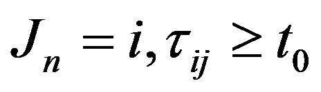 ); Dt is the discrete time when the prediction can be obtained.
Once distribution functions  have been defined and
 , Equation (4) results in:
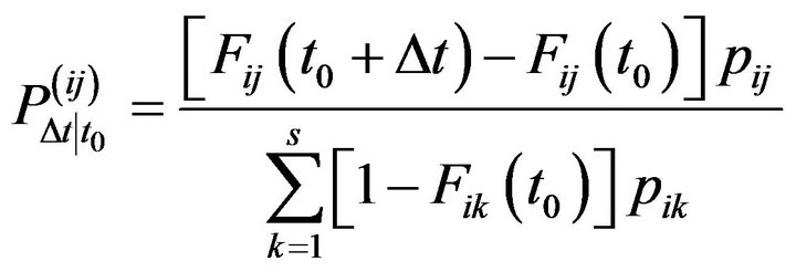 (5)
(5)
Experimental observations give the probabilities  using the ratio:
 (6)
(6)
2.3. Deterioration Process as a MRP
The stress value s recorded and evaluated at every monitoring stage is the random variable chosen for describing the deterioration process of the here proposed system. It is the ratio between the internal forces and the deteriorated area of the members’ cross-sections. Referring to Markov renewal model, the time evolution modeling of such variable need for the following assumptions [5]:
• The structure is undamaged at the initial time .
.
• The damaged structure is considered to be in a state  when
when , where
  and
and  are the lower and upper thresholds, respectively, which characterize the state i.
• The structure evolves from a state to another state
 , characterized by a lower level of performance
 ,
,  , over a time interval τij. Of course, the condition
 , with
 , is also possible if some maintenance is performed.
Under the hypothesis of MRP, the time evolution of structural behavior is then represented as transitions between different states of performance.
Choosing an appropriate PDF, the waiting time τij has been modeled for each transition. This choice is not simple and it may be “not unique”. It should be made on the basis of physical knowledge of phenomenon and on the characteristics of the distribution in their tail area where, usually, not much data are recorded.
Physical knowledge suggests that the deterioration follows a damage law that increases over time; therefore the distributions satisfying this tendency are distributions with increasing hazard rate functions 
 (7)
(7)
Although Weibull distributions and Gamma distributions are distributions characterized by a time-dependent increasing hazard rate function, their behavior is quite different. Regarding Weibull distributions at the increasing of t, with t ® ¥, the function  tends to an infinite value. Otherwise, considering Gamma for t ® ¥, the function
  tends to an asymptotic value. Then applying the abovementioned general knowledge to the case-study here discussed, for Weibull it comes out that higher is the waiting time spent by the system into the present state i highest the immediate transition into another state of j with lower performance (alert for an immediate failure). Whereas for Gamma we have that higher is the waiting time in the state i highest is the probability of transition but it tend to become almost constant (alert for a probable failure).
Experimental data recorded and their modeling brings out that the most probable behavior is the one modeled by a Gamma distribution (Figure 1).
Basing on previous considerations, a Gamma distribution has been chosen in order to model the waiting times τij. The density of the Gamma distribution is:
 , (8)
, (8)
where the shape parameter aij and the inverse scale parameter  (rate parameter) are positive parameters.
Thus, though without great emphasis, rare events within the distribution tail have been taken into consideration. After a long waiting time τij, if the transition from the state i into j isn’t occurred yet, the occurrence probability in the next Δt increases with a rise in time, τij. Anyway since values usually refer to a quasi-assured occurrence, the probability never tends to an infinite value.
Although the credibility, or validation, of one model on another is a relevant and largely debated topic [20-22] and mainly one the authors deals with it [23] the issue hasn’t been examined in this paper.
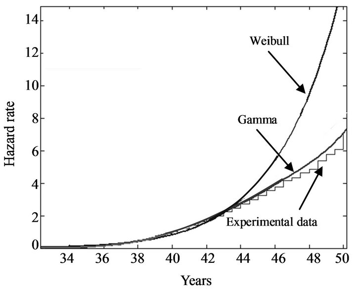
Figure 1. Comparison between hazard rate behaviors in the experimental evidence modeling.
The maximum likelihood estimates for the parameters pij, aij, rij, here presented results maximizing the loglikelihood (3) over the time window [0,T]. Using a computer code, where the routine ROSE of IMSL Fortran Library, involving the Rosenbrock’s optimization method, was implemented, the maximum likelihood assessment has been performed.
3. Deterioration Modeling
Materials deterioration due to aggressive environments or material fatigue compromises the performance of a structural system and its reliability over time. Moreover damage induced by environmental attacks suffers from uncertainty and requires to be appropriately modeled. In the following, a general approach for deterioration modeling of structural members is proposed [17].
Damage Index
Assuming Q as a generic material property, its deterioration over time t is expressed below:
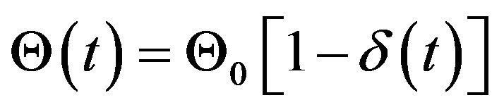 (9)
(9)
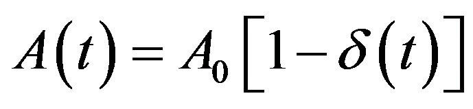
where 0 denotes the initial undamaged state, and the deterioration over time t is measured by a time-variant damage index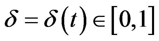 . The following damage model is assumed [17]:
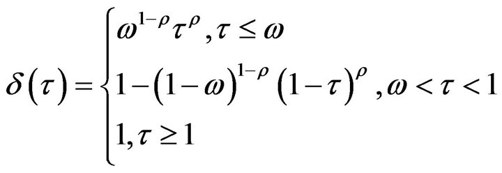 (10)
(10)
where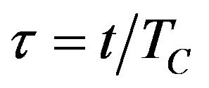 ,
,  is the normalized time instant of reaching the failure threshold
 , w and r are damage parameters defining the shape of the damage curve.
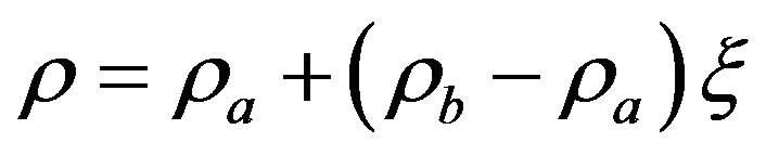
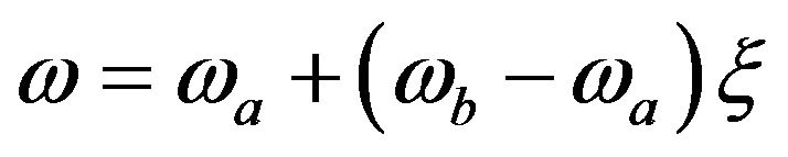
The damage parameters r and w must be chosen according to the actual evolution of the damage process. Damage rates may be associated with the aggressiveness of the environment, as well as with the active stress level.
The following linear relationship is assumed [17]:
 (11)
(11)
 (12)
(12)
where subscript a refers to damage associated with environmental aggression, subscript b refers to damage associated with loading effects, and x refers to the ratio between the level of active stress and the limit state value.
In this way, the damage law proposed is able to represent damage mechanisms induced by environmental deterioration, like carbonation of concrete, corrosion of steel or material fatigue. Generally, these mechanisms are present and interacting, and a proper calibration of the damage parameters is required based on experimental observations and/or laboratory accelerated test data.
4. Application
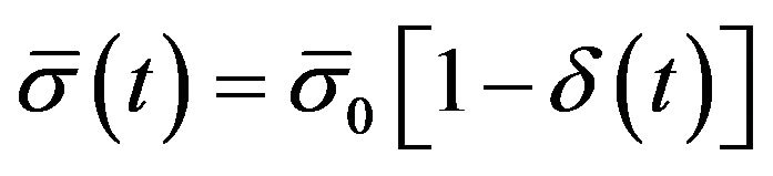
Attention is focused on truss systems subjected to a deterioration process involving a reduction of both the crosssectional area A and material strength  of each structural member. Without loss of generality, in this study it is assumed that these properties undergo the same damage process:
 (13)
(13)
 (14)
(14)
where 0 denotes the initial undamaged state, and the damage rates may be associated with the aggressiveness of the environment, as well as with the level of acting stress s with respect to the material strength , or
, or . The damage model assumed is Equation (10).
Application is made on a statically indeterminate truss system with a members’ area of A = 2500 mm2 and total volume of V = 0.0723 m3. The allowable material strength is  140 MPa. Buckling failures are assumed to be avoided. The structure is subjected to a set of forces F = 25 kN as shown in Figure 2. The initial value of the member cross-sectional area A and of the material strength
 , as well as the force F are assumed as deterministic.
Each probabilistic approach requires several experi-
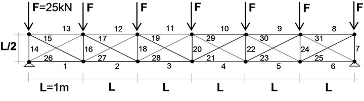
Figure 2. Statically indeterminate truss system with member area A = 2500 mm2 and total volume V = 0.0723 m3.
mental data, which are usually difficult to collect. Using the Monte Carlo simulation the samples were obtained. Based on prescribed probability distribution, the simulation process models the damage parameters ra, rb, ωa, ωb, and TC, as random variables. Considering physical knowledge of phenomena investigated, each distribution has been chosen. Starting from a mean and standard deviation, the model was defined [24,25].
Each probabilistic approach requires several experimental data that is usually difficult to collect. In this study, the samples were obtained by using the Monte Carlo simulation. In this simulation process the damage parameters ra, rb, ωa, ωb, and TC, are modeled as random variables with a prescribed probability distribution. Each distribution is chosen on the basis of physical knowledge of phenomena investigated and the model is made starting from a mean and standard deviation [24,25].
During its life the structure moves into different service states; here three different states are assumed: State 1 relates to low damage, State 2 relates to moderate damage and State 3 relates to heavy damage. The boundaries of the states are chosen on the basis of expert judgment and are presented in Table 1.
For each simulation cycle, a time-variant structural analysis is carried out by updating step-by-step updating of the stiffness matrix of the deteriorated structural members. Referring to the limit state i,  , when a member reaches the upper bound
 ![]() of the state i, the system’s transition occurs when a member reaches the upper bound
of the state i, the system’s transition occurs when a member reaches the upper bound ![]() of the state i. For each transition the crossing time is recorded and it is interpreted as the waiting time tij spent by the system in state i before the transition into the next state j.
of the state i. For each transition the crossing time is recorded and it is interpreted as the waiting time tij spent by the system in state i before the transition into the next state j.
Considering the deterioration process, if the states are significant, the transition can move state by state, otherwise the transition can involve two or more states; in other words, the transition can pass through two or more states at each step. It is clear that the choice of the size of the state is crucial and it can compromise the model. In the case study proposed, the transition always occurs state by state until failure.
With reference to the limit state , the system failure is reached when the number of failed members is able to activate a mechanism. The time in which the failure occurs is called failure time. Furthermore whenever the system reaches a given damage threshold,
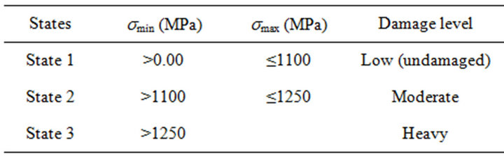
Table 1. State boundaries.
the time to reach this threshold value is called crossing time.
Then the abovementioned probabilistic approach has been applied to probabilistically investigate the next transition of the system, from the actual state i since t0 to the state j in the next interval Δt. Basing on MC simulation, a population of 5000 samples has been built. For each sample, the failure time and the crossing time related to each damage threshold have been recorded and modeled with Gamma distributions (Equation (8)). Following Equation (5), the probabilities 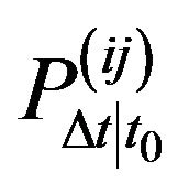 are evaluated. Since the transition between i and j could be imminent, probabilities
  with
with of
of  (n = positive number) are assumed to be dangerous for the structure. Therefore maintenance should be planned at instants close to which this probability is recorded.
5. Selective Maintenance Schedules
Generally, for maintaining two approaches can be performed:
1) Repairing all damaged members: the initial system reliability is fully restored and next maintenance can be applied at constant time intervals.
2) Repairing several damaged members: the initial system reliability is only partially restored.
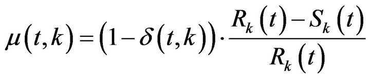
The application of the MRP can lead to decide “When to operate” but not “Where to operate”. However, considering complex structural systems, it is crucial to decide which members require maintenance. Otherwise investigating where to repair scenarios just involves the deteriorated members. Selective maintenance requires suitable life-cycle performance indicators able to select among the whole system which members require maintenance. To achieve this aim, Biondini et al. in 2008 have pointed out the following condition index m has been defined [17]:
 (15)
(15)
where d is the damage index, 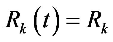 is the limit strength assumed for each member k, and
  is the corresponding loading demand. The index
  can be evaluated for each member k at each t-time over the structure’s lifetime. Basing on a suitable threshold μmin, the condition
 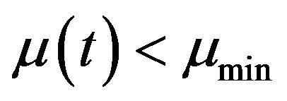 can be used to identify members which are seriously deteriorated and/or characterized by a low safety-margin.
Considering results provided by the reliability analysis, different maintenance strategies can be scheduled and different maintenance scenarios can be investigated.
In MRP the initial process instant (i.e. initial state) is relevant. Therefore if the system is new and State 1 = undamaged is the initial state, or the system is an existing building and the initial state is a generic damaged state k, the application of the method changes.
For new buildings, when the probability  reaches a value less than or equal to
 , maintenance can be performed on the whole system or on some members with a m less than a certain value. Thence the system will return to State 1 = undamaged or will be improved in a service state of major performance. The next maintenance depends on the state reached by the system after it. Then the next transition process will be modeled again as MRP.
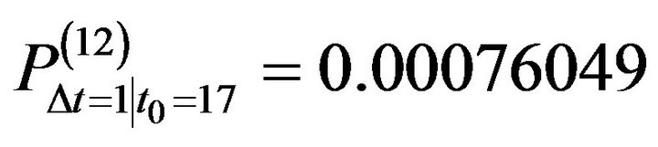
Considering previous observations, the life-cycle assessment of the system in Figure 2 has been performed. Supposing the system “new” and assuming t0 initially equal to zero and the State 1 undamaged, Equation (5) describes the occurrence of the transition probability from State 1 to State 2, i.e. 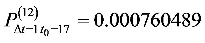 in the next year (Δt = 1) after 17 years of construction (t0 = 17). Furthermore the transition from State 2 into State 3 could occur 2 years after the last transition with a probability
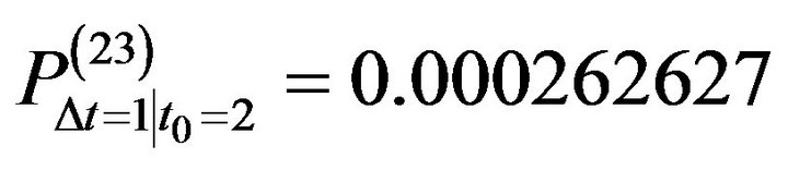 . When the structure is 25 years old, the prediction of failure in the following year becomes very probable,
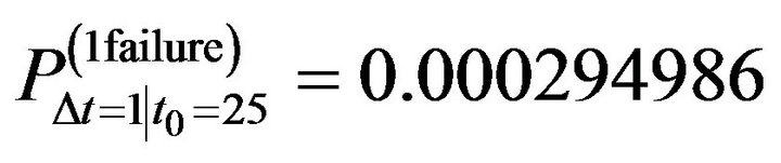 .
.
Therefore, maintenance scenarios involve:
a) The repair of the whole system after 17 years of construction. The system will return to State 1 = undamaged, the deterioration process becomes a renewal process and maintenance will be carried out every 17 years.
b) The repair of the whole system at the time of failure (25 years). The process becomes again a renewal process.
c) The repair of just some members of the system will move it into a state j equal or different to the initial state State 1 = undamaged. The next maintenance will occur with t0 difference in comparison to the initial one (ex.: t0 = 11 years). The process can be modeled again as a MRP and the new probability of transition is investigated. Considering this scenario, the use of condition index m is crucial.
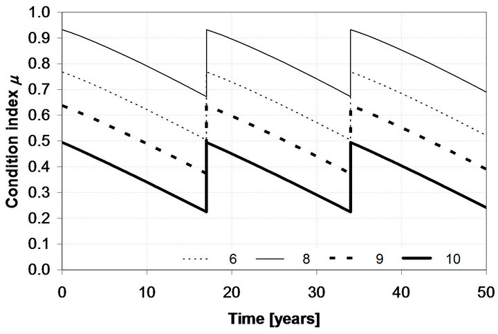
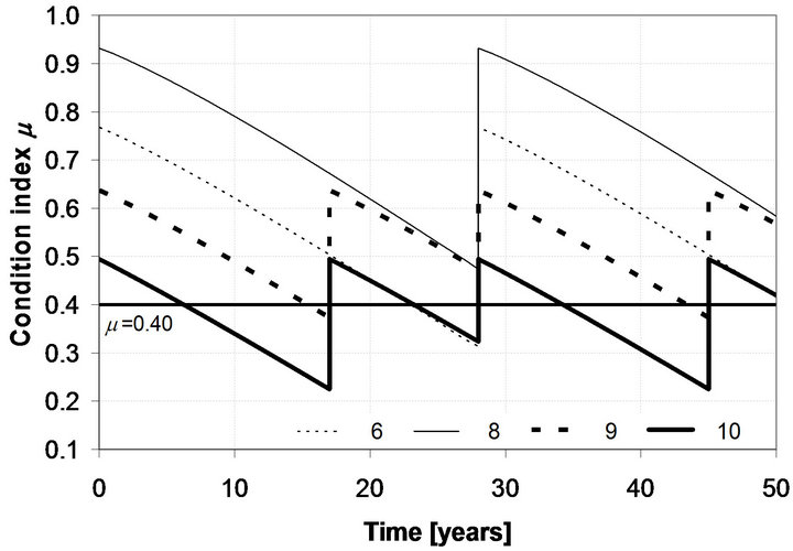
Figure 3 shows the comparison between the behaviors of the survival functions  of scenarios a) and b) over the system’s service life. Whenever maintenance is carried out, the system renews itself and the process restarts with the same survival function. Concerning scenarios a) and b), Figure 4 shows the condition index’s behavior over the life of some members of the system when the danger limits assumed are
 and
and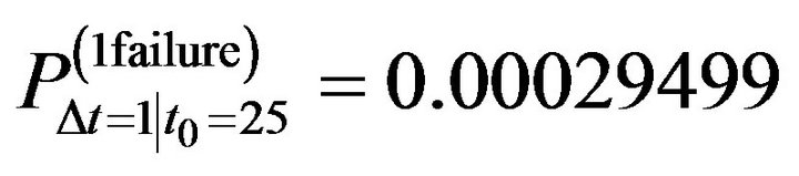 respectively.
Scenario c) enables to propose several other possible scenarios connected with selective maintenance and
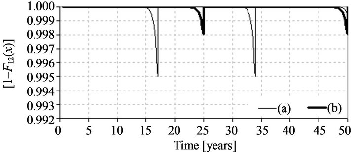
Figure 3. Comparison between survival functions of scenario (a) and (b) throughout system’s service life; in both the scenarios when maintenance is carried out the system renews itself.
 (a)
(a)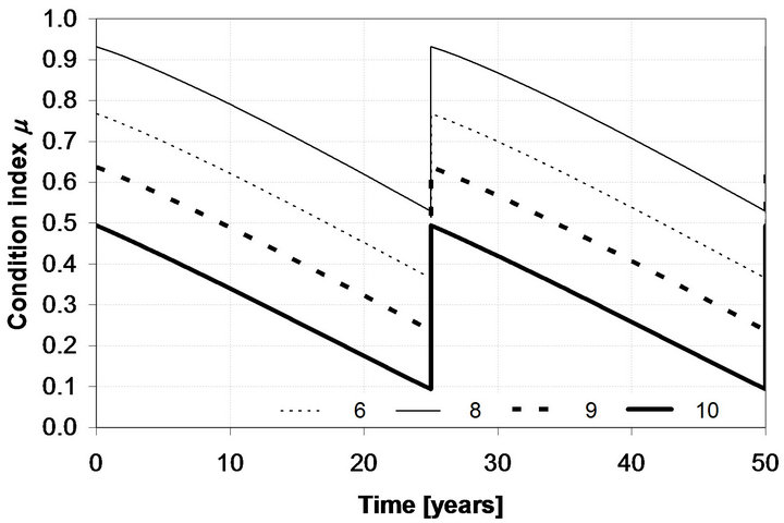 (b)
(b)
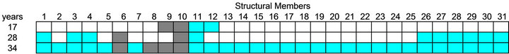
Figure 4. Condition index’s behavior for scenario (a) and scenario (b) throughout the service life and concerning members 6, 8, 9 and 10 of the system.
supported by the behavior of condition index m. Thus, for instance, the first scenario (scenario (1)) foresees maintenance performed after 17 years
 on those members with a condition index
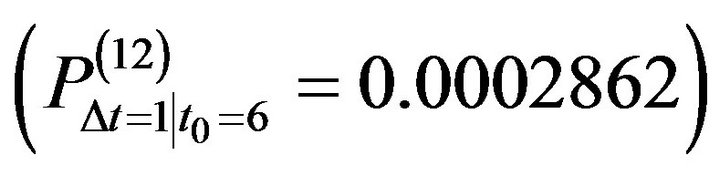
 . This maintenance moves the system from State 2 into State 1 = undamaged, but the probability of the next transition into State 2 is higher than the probability connected with the new system. MRP suggests that the new transition into State 2 could happen in Dt = 1 year and t0 = 11 years with a probability
 .
.
At the new transition (11 year after the first one) there are 12 members with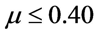 ; once again it seems to be convenient to replace only these twelve members.
After maintenance, the system moves from State 2 into State 1. Running a new Monte Carlo simulation and applying MRP, the occurrence of the new transition from State 1 into State 2 just 6 years after the last maintenance
 comes out. Furthermore a replacement of the whole system is necessary. Since maintaining the whole system after 6 years may be not convenient, scenario (2) is approached. In this case the maintenance of the whole system is performed at the 28th year and the system renews itself after the second maintenance.
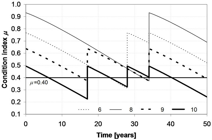
Figure 5 shows the comparison between the behavior of the survival functions for scenarios (1) and (2) through the service life of the system. Assuming a danger limit threshold of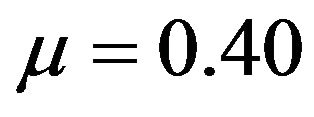 , the time-dependent behavior of the condition index concerning some of the members has been investigated (Figure 6).
6. Maintenance Cost
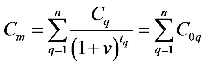
Each maintenance scenario considered must be conveniently associated to maintenance cost. Considering a prescribed maintenance scenario, the total cost of maintenance Cm can be estimated as the sum of the costs Cq of the individual interventions [18],
 (16)
(16)
where the cost Cq of the qth rehabilitation depends on the initial time of construction with a properly discounted rate of money v [18]. The cost Cq of the individual intervention is assumed as follows:
 (17)
(17)
where  is a fixed cost computed as a percentage a of the initial cost C0, dk is the damage index of member k belonging to the structural system, Vk is the volume of member k, and cqk is the volume unit cost for restoring member k.
Basing on this cost model, different maintenance scenarios can be economically compared and optimal maintenance strategies can be selected [3,4,17].
Firstly scenario (a) (Figure 4(a)) is compared with scenario (b) (Figure 4(b)). Figure 7 shows the total cost Ca, computed as the sum of initial cost C0 and maintenance cost Cm of scenario (a) normalized to the cost Cb of scenario (b), 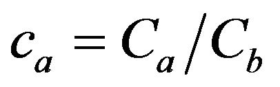 , versus the discount rate n, for different values α of the fixed cost of maintenance,
 . Considering a discount rate n less than 0.04
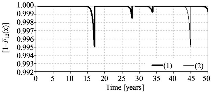
Figure 5. Comparison between survival functions of scenario (1) and (2) throughout the service life; when maintenance is carried out the system returns to initial state.
Scenario (1)
Scenario (2)
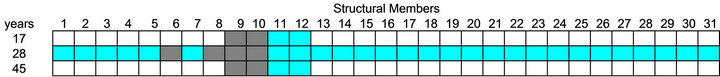
Figure 6. Condition index’s behavior for scenario 1) and scenario 2) throughout the service life and concerning members 6, 8, 9 and 10 of the system. The table below the figures shows the members replaced at every maintenance action. The members are pinpointed in dark gray.
and a percentage a less than 0.15, the economic primacy of scenario (a) over scenario (b) is evident. For  (no fixed cost admitted) scenario (a) is the most convenient one.
When maintenance is performed, scenario (b) always requires the replacement of the 99% of the system’s volume in order to return the system to initial condition.
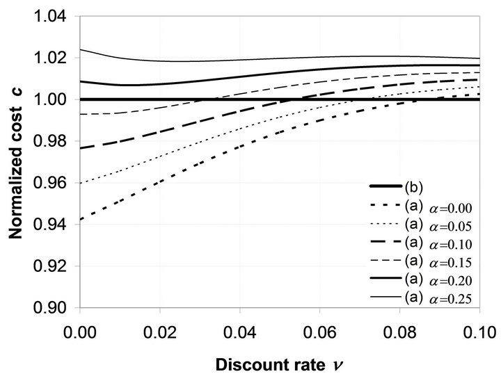
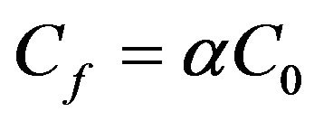
Figure 7. Total cost Cb, computed as the sum of initial cost C0 and maintenance cost Cm, of scenario (b) normalized to cost Ca of scenario (a), or ca = Ca/Cb versus the discount rate n, for different values a of the fixed cost of maintenance Cf = aC0.
Anyway, just one maintenance is scheduled over the system’s life cycle. Scenario (a) requires a 40%-replacement of the system’s volume otherwise. In this case two maintenance actions must be planned. Thence scenario (a) becomes less convenient when the fixed costs connected with each maintenance action become significant.
Figure 8 compares scenario (1) and scenario (2). The behavior of the total cost, C2, of scenario (2), normalized to the cost, C1, of scenario (1), versus the discount rate, n, for different values α of the fixed cost of maintenance Cf = aC0 has been presented. The economic primacy of scenario (2) over scenario (1) has been pointed out. Besides, scenario (2) is less sensitive to a value and seems to confirm that a renewal with two maintenance actions is better, especially with a discount rate close to 0.03.
7. Conclusions
The main features of a method for life-cycle reliability assessment as well as for the maintenance schedule of deteriorating structural systems have been proposed. Basing on the effective modelling of structural damage and using a Markov Renewal Process, this procedure enables to model the deterioration process as a transition process through performance states. For supporting the MRP with experimental data, a Monte Carlo simulation is introduced. The Monte Carlo simulation collects many samples and provides a significant population for a probabilistic approach. The next step of this research will develop a validation for this probabilistic approach.
This paper proposes a definition of a condition index which identifies selective maintenance scenarios, where repair interventions are only applied to seriously deteriorated members and/or elements characterised by a low safety-margin.
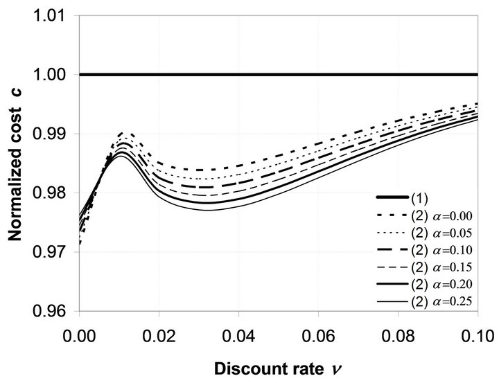
Figure 8. Total cost C2, computed as the sum of initial cost C0 and maintenance cost Cm, of scenario (2) normalized to cost C1 of scenario (b), or c2 = C2/C1 versus the discount rate n, for different values a of the fixed cost of maintenance Cf = aC0.
The method here presented is applied to compare different maintenance scenarios, where maintenance is performed as selective maintenance or total maintenance of the system. The results prove the convenience of carrying out maintenance before reaching the failure threshold just within not relevant fixed cost of maintenance.
8. Acknowledgements
The authors are grateful to Prof. Frangopol and Prof. Biondini for their help in the development of this research. The third author wishes to acknowledge the support of the Regione Lombardia within the project Dote Ricercatori.
REFERENCES
- P. G. Malerba, L. Sgambi, D. Ielmini and G. Gotti, “Influence of Corrosive Phenomena on the Mechanical behaviour of R. C. Elements,” Proceedings of 2011 World Congress on Advances in Structural Engineering and Mechanics, Seoul, 18-22 September 2011, pp. 1269-1288.
- L. Sgambi, F. Bontempi and E. Garavaglia, “Structural Response Evaluation of Two-Blade Bridge Piers Subjected to a Localized Deterioration,” Proceedings of the 3rd International Conference on Bridge Maintenance, Safety and Management, Porto, 16-19 July 2006, pp. 153- 154.
- F. Biondini, F. Bontempi, D. M. Frangopol and P. G. Malerba, “Probabilistic Service Life Assessment and Maintenance Planning of Concrete Structures,” Structural Engineering, Vol. 132, No. 5, 2006, pp. 810-825. doi:10.1061/(ASCE)0733-9445(2006)132:5(810)
- F. Biondini and D. M. Frangopol, “Long-Term Performance of Structural Systems,” Structure and Infrastructure Engineering, Vol. 4, No. 2, 2008, p. 75.
- F. Biondini and E. Garavaglia, “Probabilistic Service Life Prediction and Maintenance Planning of Deteriorating Structures,” Proceedings of International Conference on Structural Safety and Reliability, Rome, 19-22 June 2005, pp. 495-501.
- R. A. Howard, “Dynamic Probabilistic Systems,” John Wiley and Sons, New York, 1971.
- N. Limnios and G. Oprisan, “Semi-Markov Processes and Reliability,” Birkhauser, Boston, 2001. doi:10.1007/978-1-4612-0161-8
- E. Alvarez, “Estimation in Stationary Markov Renewal Processes, with Application to Earthquake Forecasting in Turkey,” Methodology and Computing in Applied Probability, Vol. 7, No. 1, 2005, pp. 119-130. doi:10.1007/s11009-005-6658-2
- I. Votsi, N. Limnios, G. Tsaklidis and E. Papadimitriou, “Estimation of the Expected Number of Earthquake Occurrences Based on Semi-Markov Models,” Methodology and Computing in Applied Probability, Vol. 14, No. 3, 2012, pp. 685-703.
- G. Masala, “Hurricane Lifespan Modeling through a Semi-Markov Parametric Approach,” Journal of Forecasting, Online, 2012.
- G. Masala, “Earthquakes Occurrences Estimation through a Parametric Semi-Markov Approach,” Applied Statistics, Vol. 39, No. 1, 2011, pp. 81-96.
- E. Garavaglia and R. Pavani, “About Earthquake Forecasting by Markov Renewal Processes,” Methodology and Computing in Applied Probability, Vol. 13, No. 1, 2011, pp. 155-169. doi:10.1007/s11009-009-9137-3
- E. Garavaglia, E. Guagenti, R. Pavani and L. Petrini, “Renewal Models for Earthquake Predictability,” Journal of Seismology, Vol. 14, No. 1, 2010, pp. 79-93. doi:10.1007/s10950-008-9147-6
- E. Garavaglia, A. Gianni and C. Molina, “Reliability of Porous Materials: Two Stochastic Approaches,” Journal of Materials, Vol. 16, No. 5, 2004, pp. 419-426. doi:10.1061/(ASCE)0899-1561(2004)16:5(419)
- E. Garavaglia, A. Anzani, L. Binda and G. Cardani, “Fragility Curve Probabilistic Model Applied to Durability and Long Term Mechanical Damages of Masonry,” Materials and Structures, Vol. 41, No. 4, 2008, pp. 733-749. doi:10.1617/s11527-007-9277-2
- A. Anzani, E. Garavaglia and L. Binda, “Long-Term Damage of Historic Masonry: A Probabilistic Model,” Construction and Building Materials, Vol. 23, No. 2, 2009, pp. 713-724. doi:10.1016/j.conbuildmat.2008.02.010
- F. Biondini, D. M. Frangopol and E. Garavaglia, “LifeCycle Reliability Analysis and Selective Maintenance of Deteriorating Structures,” Proceedings of 1st International Symposium on Life-Cycle Civil Engineering, Varenna, 10-14 June 2008, CRC Press, Taylor & Francis Group, London, 2008, pp. 483-488.
- J. S. Kong and D. M. Frangopol, “Life-Cycle ReliabilityBased Maintenance Cost Optimization of Deteriorating Structures with Emphasis on Bridges,” Structural Engineering, Vol. 129, No. 6, 2003, pp. 818-824. doi:10.1061/(ASCE)0733-9445(2003)129:6(818)
- D. R. Cox, “Renewal Theory,” Methuen Ltd., London, 1962.
- D. Vere-Jones, D. Harte and M. Kosuch, “Operational Requirements for an Earthquake Forecasting Programme in New Zealand,” Bulletin of the New Zealand National Society for Earthquake Engineering, Vol. 31, 1998, pp. 194-205.
- G. Grandori, E. Guagenti and A. Tagliani, “A Proposal for Comparing the Reliabilities of Alternative Seismic Hazard Models,” Journal of Seismology, Vol. 2, No. 1, 1998, pp. 27-35. doi:10.1023/A:1009779806984
- G. Grandori, E. Guagenti and A. Tagliani, “Magnitude Distribution versus Local Seismic Hazard, BSSA,” Bulletin of Seismological Society of America, Vol. 93, No. 3, 2003, pp. 1091-1098.
- E. Garavaglia, “The Credibility Measure of Probabilistic Approaches in Life-Cycle Assessment of Complex Systems: A Discussion,” Materials with Complex Behaviour II, Öchsner, et al., Eds., Springer-Verlag, Berlin, 2012, pp. 619-636. doi:10.1007/978-3-642-22700-4_38
- M. Ciampoli, “A Probabilistic Methodology to Assess the Reliability of Deteriorating Structural Elements,” Computer Methods in Applied Mechanics and Engineering, Vol. 168, No. 1-4, 1999, pp. 207-220. doi:10.1016/S0045-7825(98)00141-8
- A. Gupta and C. Lawsirirat, “Strategically Optimum Maintenance of Monitoring Enabled Multi-Component Systems Using Continuous-Time Jump Deterioration Models,” International Conference on Simulation and Modeling, Bankgok, 17-19 January 2005, pp. 306-329.