Applied Mathematics
Vol. 3 No. 11A (2012) , Article ID: 24764 , 9 pages DOI:10.4236/am.2012.331250
LSFEM Implementation of MHD Numerical Solver
1University J. E. Purkinje, Ústí nad Labem, Czech Republic
2Max Planck Institute for Solar System Research, Katlenburg-Lindau, Germany
3Astronomical Institute of Czech Academy of Sciences, Ondřejov, Czech Republic
Email: barta@asu.cas.cz, miroslav.barta@mpi-sf.mpg.de
Received August 7, 2012; revised September 8, 2012; accepted September 16, 2012
Keywords: Magnetohydrodynamics (MHD); Least-Squares Finite Element Method; Adaptive Mesh Refinement; Magnetic Reconnection; Solar Eruptions; MHD Turbulence
ABSTRACT
Many problems in physics are inherently of multi-scale nature. The issues of MHD turbulence or magnetic reconnection, namely in the hot and sparse, almost collision-less astrophysical plasmas, can stand as clear examples. The Finite Element Method (FEM) with adaptive gridding appears to be the appropriate numerical implementation for handling the broad range of scales contained in such high Lundquist-number MHD problems. In spite the FEM is now routinely used in engineering practice in solid-state and fluid dynamics, its usage for MHD simulations has recently only begun and only few implementations exist so far. In this paper we present our MHD solver based on the Least-Square FEM (LSFEM) formulation. We describe the transformation of the MHD equations into form required for finding the LSFEM functional and some practical issues in implementation of the method. The algorithm was tested on selected problems of ideal (non-resistive) and resistive MHD. The tests show the usability of LSFEM for solving MHD equations.
1. Introduction
Dynamics of magnetized plasma at sufficiently large spatial and temporal scales can be adequately described by the set of magnetohydrodynamic (MHD) equations [1]. In many problems we face the situation with high Lundquist (a.k.a. magnetic Reynolds) number
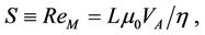
where L is the characteristic size of the system,  the typical Alfvén velocity (B and
  being the magnetic field strength and plasma density, respectively) and
  the electric resistivity. A direct consequence of the high Lundquist number is a large separation between the system size and the dissipation scale. The cascading fragmentation of the current layer in the magnetic reconnection in solar flares [2-4] can serve as an example of such a multi-scale problem: The span between the eruption size (
 km) and the dissipation scale (1 m - 10 m) in the practically collision-less coronal plasmas easily extends seven orders of magnitude.
In general, there are two approaches how to handle such a broad range of scales. The first one uses a moderate numerical resolution and models the physics on the sub-grid (unresolved) scales using some plausible assumptions on the micro-scale statistical properties (correlations) of the quantities that define the system (e.g. flow or magnetic field). Among them, e.g., the LargeEddy Simulations (LES) [5] or Reynolds-Averaged Numerical Simulations (RANS) [6] belong to the well known methods used widely in engineering applications in the fluid dynamics.
The second approach is based on direct simulations that cover all the scales contained in the problem. Traditionally, the Adaptive Mesh Refinement (AMR) technique is used with the Finite-Difference/Finite Volume Methods in order to resolve high-gradient regions locally, keeping the total number of grid points required for simulation at a manageable level [7-9]. Nevertheless, also this approach has its limitations caused by introduction of artificial boundaries between fine and coarse meshes. This problem, however, can be cured by the methods based on unstructured mesh, such as is used in FEM. With this in mind we have implemented a FEM-based solver for MHD equations and present it in the current paper. From various FEM formulations we have chosen the LSFEM because it is robust, universal (it can solve all kinds of partial differential equations) and it is efficient—it always leads to the system of linearized equations with symmetric, positive definite matrix [10]. The LSFEM keeps many key properties of the Rayleigh-Ritz formulation even for systems of equations for which the equivalent optimization problem (in Rayleigh-Ritz sense) does not exist [11].
Despite of the FEM applications in the fluid dynamics made a substantial development in the past years, its usage for numerical solution of MHD equations is still rather rare. For example, the NIMROD [12] and M3D codes [13]—based on Galerkin formulation—belong to a few known implementations of FEM-based MHD solvers. Related work also has been done by [14] who implemented the MHD (and two-fluid) equations within the more general code framework SEL [15] based on the Galerkin formulation with high-order Jacobi polynomials as the basis functions. However, to our knowledge, the LSFEM implementation of the MHD solver described in the current paper is the first attempt of this kind.
The paper is organized as follows: First, we briefly describe the underlying MHD model. Then, the MHD equations are re-formulated in the general flux/source (conservative) formulation. Temporal discretization, reduction to the first-order system, and linearization procedure are described subsequently. Then, the properties of the least-square formulation of FEM are briefly summarized. Some practical arrangements of the LSFEM implementation of the MHD solver follows. Finally, the code is tested on a couple of standardized model problems and the results are discussed with respect to the intended application of the code to the current-layer filamentation and decay during the magnetic reconnection in solar eruptions.
2. MHD Equations
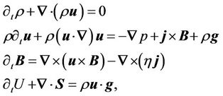
The large-scale dynamics of magnetized plasma can be described by MHD equations for compressible resistive fluid [1]:
 (1)
(1)
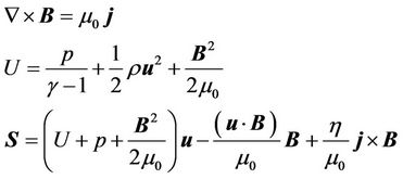
where ρ, v, B, U are density, macroscopic velocity, magnetic field, and total energy density, respectively, g being the gravity acceleration. The energy flux S and auxiliary variables j (current density) and p (plasma pressure) are given by the following relations:
 (2)
(2)
In the (almost) collision-less plasma, in which we are mostly interested, the classical resistivity usually plays a small role. Instead of that various microscopical (kinetic) effects influence the plasma dynamics via other terms in the generalized Ohms law [16]. In order to mimic these processes, whose modeling is beyond the scope of MHD approach, we re-consider the parameter  as a generalized resistivity, including the effects like wave-particle interactions or off-diagonal components in the electron pressure tensor into it. As such effects are—in general— observed in the highly filamented, intense current sheets we model the anomalous generalized resistivity as follows:
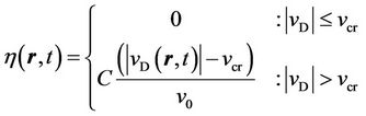 (3)
(3)
Thus, the non-ideal effects are turned on whenever the current-carrier drift velocity
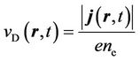 (4)
(4)
exceeds the critical threshold .
.
In order to solve the Equation (1) numerically, it is convenient to rescale all the quantities into the dimensionless units. Thus, all the spatial coordinates are expressed in the characteristic size L and times in Alfvén transit time , where
 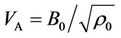 is a typical Alfvén speed. Magnetic field strength B and plasma density
  are given in units of their characteristic values
  and
and  and similar scaling holds for the other quantities—see [17] or [3] for details. From now on we shall use this dimension-less system.
In order to utilize a more universal LSFEM implementation for more general form of equations (c.f. with SEL approach [14]) the set of MHD Equation (1) is rewritten into the conservative (flux/source) formulation:
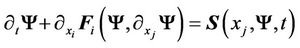 (5)
(5)
Here the local state vector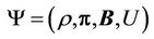 ,
,  being the momentum density. The flux
  and the source-term
  are defined as
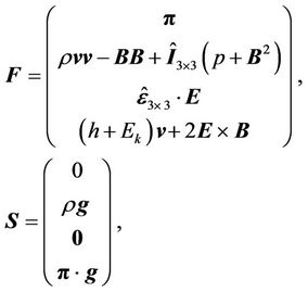 (6)
(6)
where  is the
  unit matrix,
  is the permutation pseudo-tensor,
 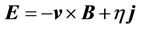 is the electric field strength. The the enthalpy and kinetic energy densities are
 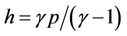 and
and , respectively.
3. FEM Formulation of MHD System
In general, FEM is formulated for the linear problem
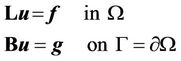 (7)
(7)
where L is the linear (differential) operator, B the boundary operator,  is the domain and
  is the boundary of
 .
.
In order to reformulate the system of Equations (5) into the standardized problem (7) several steps have to be undertaken. First of all, we perform the time discretization. We use the standard  -differencing scheme (see [18]):
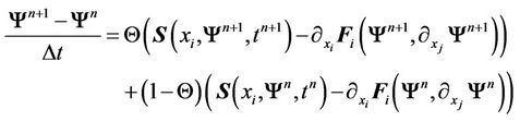 (8)
(8)
where parameter  controls the implicitness of the scheme, and n and
  designate the old and new time-steps, respectively. The scheme leads to the following semi-implicit equation
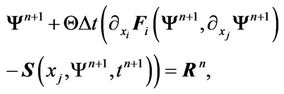 (9)
(9)
where the RHS vector  consists of components known at old time step.
Since practical implementations of LSFEM require first order system of PDEs [10,11] we further transform the system (5) to the required form introducing a new independent system variable—the electric field
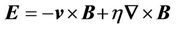 (10)
(10)
The procedure is basically analogous to the velocityvorticity formulation of the Navier-Stokes equations in the CFD.
A frequent problem in the numerical MHD is a violence of the solenoidal condition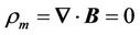 , where the (dummy) variable
  represents the artificial density of the magnetic charge. The advantage of the LSFEM implementation is that this constraint can be directly included into the set of the governing equations [10]. Then assembling the solenoidal condition together with Equations (9) and (10) we arrive to the following 1st-order vector equation for our modeled system:
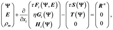 (11)
(11)
where all the LHS terms are evaluated in the advanced time-step . Here,
  and
and  are given by Equation (6) with
  considered as an independent variable now and
 . The fluxes
 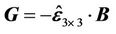 and
and  imply from Equation (10) and the solenoidal condition. The source term component
 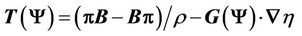 . We keep the artificial magnetic-charge density
  at zero.
Equation (11) can be written in the conservative form similarly as in Equation (5)
 (12)
(12)
with the extended state vector, fluxes and source terms in the form
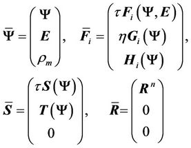 (13)
(13)
Since the extended flux  and source term
  depend non-linearly on the state vector
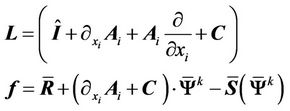
 , a linearization procedure has to be applied in order to transform the system (12) into the FEM-conforming form (7). We use the standard Newton-Raphson (NR) iterations in each time step [10,19]. Thus, the flux at the NR iteration
  can be expressed as [18]:
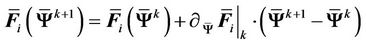 (14)
(14)
and analogous expression holds for the source term. Introducing the Jacobians
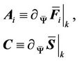 (15)
(15)
the final equation for NR iterations reads
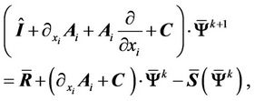 (16)
(16)
where the RHS contains only the terms from the  th iteration of the currently solved time-step
  and variables known at the previous step
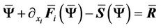
 . Equation (16) is already in the form (7) with
 (17)
(17)
4. LSFEM Implementation
In the least-square formulation of the FEM the problem described by Equation (7) is transformed to seeks the minimum of the functional
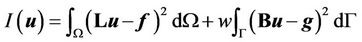 (18)
(18)
where w is appropriate mesh-dependent weighting factor [11]. As in other FEM implementations, the solution is searched for in a limited subspace of functions that are formed as a union of the piece-wise functions  defined on a single, in our code triangular element, as a linear combination of the basis functions
 :
:
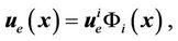 (19)
(19)
where  can always represent the value of a function
  in a properly selected point (the node)
 . Here
  denotes element-wise index of the node. In our code we use Lagrangian polynomials for basis functions
 .
.
Varying the functional (18) and inserting the expansion (19) we arrive to a set of linear algebraic equations for each internal element in the form
 (20)
(20)
where  is the domain of the
  -th element in the global domain
 . The boundary elements contain additional terms obtained from the boundary operator (the second term in Equation (18)). For fast evaluation of local integrals we use Gaussian quadrature [18] in the system of element natural coordinates [20].
Equations (20) for each element are finally assembled to a global linear system of equations via mapping the element-wise node index j to a global node index N described in [18], to obtain
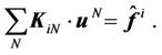 (21)
(21)
The final matrix K is sparse, symmetric and positive definite. In our code we use preconditioned Jacobi Conjugate Gradient Method (JCGM) [21] for solution of the system (21).
The entire algorithm can be summarized as follows:
− time loop—adapt time step size according to CFL condition, check final desired time
− linearization loop—if 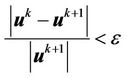 or maximum iteration count is reached continue to next time step
− assembling stiffness matrix  element by element
− integration by Gaussian quadrature
1) compute the operator matrices for each basis function 2) multiply the operator matrices then add the result into stiffness matrix 3) multiply the operator matrix by the RHS then add result into the load vector
− next Gaussian point
− next element
− find new solution  of system (21) by the JCGM
− next linearization
− next time step Thanks to the iterative nature of the JCGM, the solver algorithm can be rather easily parallelized via MPI. We decompose the entire domain into subdomains, splitting the global matrix K and the load vector  into corresponding segments with rather small overlaps related to internal-boundary nodes shared by both adjacent subdomains. Matrix multiplications are then performed only locally (per-process) and, finally, resulting global vectors are appropriately assembled using MPI operations that transfer the data related to overlapping nodes only.
5. Numerical Tests
In order to assess usability and properties of the LSFEM MHD solver we perform several tests on standardized ideal (non-resistive) and resistive MHD problems. For all test we use the adiabatic index , the implicitness parameter
  (Crank-Nicholson time discretization), and the Courant number 0.6.
5.1. Ryu-Jones Discontinuity Test Problem
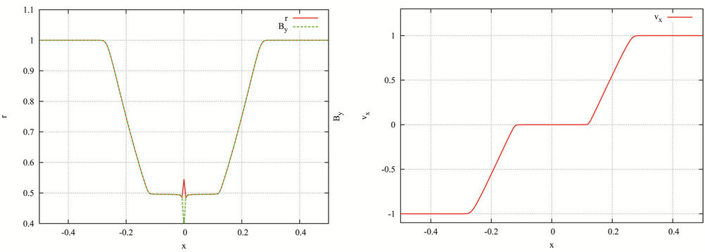
First, we applied our code onto the standard Ryu-Jones ideal MHD 1D shock/discontinuity problem [22]. The initial state is given by prescriptions 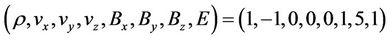 in the left half, and
 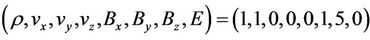 in the right half of the computational box, respectively. The domain
  was divided into 512 elements. We used the first order basis functions to approximate the FEM solution. The boundary conditions on both ends are of von Neumann type. Results at time
  are shown in Figure 1. They correspond and could be compared with Figure 3(b) in [22].
In order to study influence of basis-function order on the approximate solution we calculate the same test problem, now with the second-order Lagrange polynomials. All other parameters are the same as in the previous case displayed in Figure 1. The results are shown in Figure 2.
5.2. Orszag-Tang Vortex Test Problem
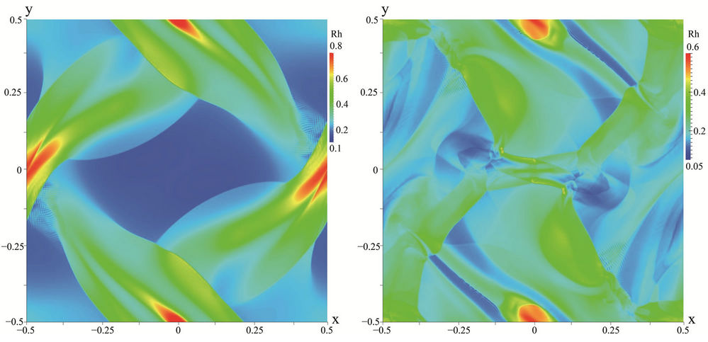
A next test we performed standard Orszag-Tang 2D ideal-MHD vortex problem [23]. The initial state was given by the following relations:

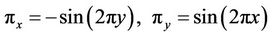
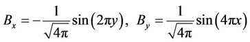

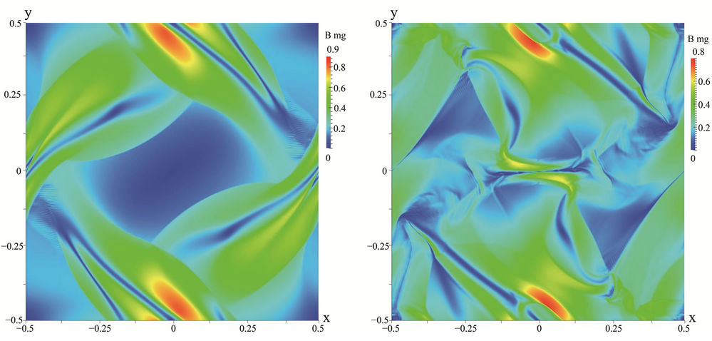
The computational domain 1.0 × 1.0 was discretized by 2 × 640 × 640 triangular elements. We apply periodic boundary conditions at all boundaries. The first-order basis functions were used in this simulation. Results in Figures 3 and 4 show the plasma density and the magnitude of the magnetic field, respectively, at times t = 0.25 (a), and t = 0.50 (b).
5.3. Resistive Decay of a Cylindric Current
In order to assess the applicability of our code to the solutions of non-ideal (resistive) MHD problems and to estimate its numerical resistivity we performed a following test: At the initial state  a cylindrical current
  with
with
 (a)
(a)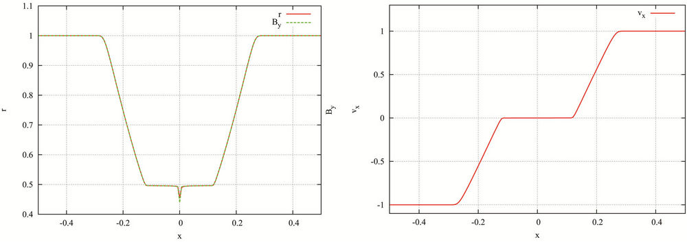 (b)
(b)
Figure 1. The LSFEM solution of the MHD shock tube test (Ryu-Jones problem) at time t = 0.1 with the first-order basis functions. (a) density profile (red dashed line) and By profile along x-axis. (b) vx profile along x-axis.
 (a) (b)
Figure 2. The LSFEM solution of the MHD shock tube test (Ryu-Jones problem) at time t = 0.1 with the second-order basis functions. Displayed quantities are the same as in Figure 1.
 (a) (b)
Figure 3. The Orzsag-Tang vortex. The color coded plasma density is displayed at time t = 0.25 (a) and t = 0.50 (b).
 (a) (b)
Figure 4. The Orzsag-Tang vortex. The color coded magnitude of the magnetic field is displayed at times t = 0.25 (a) and t = 0.50 (b).
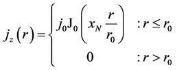
flows through a plasma of a uniform density . Here,
  is the amplitude of the current density on the cylinder axis,
  is the cylinder radius, and
  is the first null of the Bessel function of the 0th order
 . The resistivity inside the cylinder
  is uniform
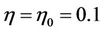 , outside
 . In order to be able to compare the numerical results with an analytical solution and to split advective and resistive properties of the code we set all velocities to zero at
  and the density to a very high value
  to keep the plasma in rest. In the limit
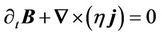
  the MHD system (1) effectively reduces into the diffusion equation
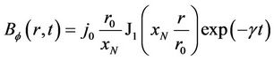
whose analytical solution for our initial state keeps the form  with
with
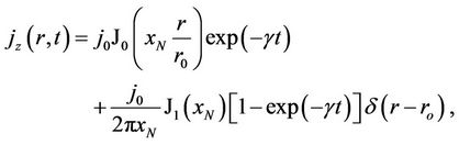 (22)
(22)
where  is the Bessel function of the 1st order and
  is the Dirac delta function. The decrement
  reads
reads
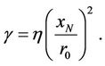 (23)
(23)
The second term in Equation (22) represents an induced surface current that compensates resistive decrease of the current density inside the column to keep the magnetic field in the outer super-conducting domain constant. The corresponding magnetic field is of the form  where
where
for internal  region and
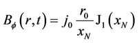
for the outer space.
Computational domain is divided into a homogeneous mesh of  triangles in our numerical test. We use the first order basis functions to approximate the numerical solution. Free boundary conditions were applied on all boundaries. The results of this test are shown in Figure 5. Figure 5(a) shows time evolution of the current density profile along
  for five subsequent time instants. Resistive decrease of
  inside the column accompanied by formation of the induced surface current are well visible. Figure 5(b) shows a comparison of numerical and analytical solutions for time evolution of the current density
  at
at ,
, .
.
6. Discussion and Conclusions
The FEM represent an alternative to FDM/FVM that are traditionally used for solution of MHD problems in astrophysics. Its attractivity implies from its unstructured mesh that allows for appropriate local refinement without formation of qualitative internal boundaries between the fine and coarse meshes. This property makes it very useful for handling the multi-scale problems, for example the problem of magnetic reconnection in solar flares [3] (and other large-scale systems) or MHD turbulence.
With this intention in mind we have developed the LSFEM implementation of a MHD solver whose descriptions and preliminary results from its application to the standardized test problems are presented in this paper.
To sum up the main points of our implementation: Transformation of the MHD equations (1) to the standard FEM problem (7) involves several steps: 1) Standard  -time discretization; 2) Decrease of the order of the system of equations by introduction of a new variable— electric field strength; and 3) Newton-Raphson linearization. The possibility to include the solenoidal condition
  directly into the system of equations certainly belongs to advantages of LSFEM formulation, as well as a natural involvement of the boundary conditions. The element-by-element assembling of the global stiffness matrix and the iterative nature of JCGM solver allow for rather easy and efficient MPI parallelization. Integrals over elements are efficiently performed via Gauss quadrature.
We performed several standardized tests focused on an
 (a) (b)
Figure 5. A resistive decay of a cylindrical current density with time. (a) profiles of jz(x, 0, t) at five subsequent times; (b) The time profile of jz(0, 0, t)-comparison of numerical and analytical [Equation (22)] solutions.
ideal and resistive MHD. The LSFEM MHD solver quite closely reproduces results published for the Ryu-Jones shock tube problem [22]. Small spurious oscillations appear around the points where the first derivative of an analytical solution does not exist. Choice of the higherorder basis functions makes the situation even slightly worse.
Similar feature can be seen in the results from the Orszag-Tang vortex test problem. While the large-scale dynamics agree well with those obtained from the “gauge” codes, small oscillations accompanying the shocks are visible again. These effects are caused by the least squares curve fitting approach [11]. We believe that it can be cured by an introduction of a small background resistivity and local refinement of the mesh around the discontinuities, with the element size corresponding to the resistivity-controlled (magnetic) Reynolds number. Such approach is fully in line with the intended usage of the code for detailed studies of the current sheet filamentation and fragmentation in a large-scale magnetic reconnection in solar flares. Indeed, in the solar corona we have a very small background classical resistivity due to (rare) collisions between electrons and ions as well. Hence, having mesh around the filamenting current sheet locally refined as much as possible we can set the background (physical) resistivity accordingly and approach thus the realistic Lundquist number in the solar corona.
Finally—with the intended usage of the code in mind —we have tested the properties of our implementation for solution of the resistive problems. In order to get a comparison with an analytical solution we have “frozen” the plasma dynamics by setting high matter density and we concentrated on a purely diffusive problem. The results show a rather good agreement with the analytical solution. Namely, the induced surface current density is located only at a few elements and did not diffuse further with time. This is an important result for intended future studies of the current-sheet filamentation in the flare reconnection.
The tests show basic applicability of our LSFEM implementation of the MHD solver for a solution of selected problems. At the same moment they reveal the necessity to involve both the adaptive spatial refinement (it has already been implemented) and adaptive change of the order of basis functions over selected elements (h-p refinement). These features will be implemented into our code in a near future.
7. Acknowledgements
This research was supported by the grants P209/12/0103 (GA  R), P209/10/1680 (GA
  R), and the research projects RVO: 67985815 (CZ) and CRC 963 (DE). M.B. acknowledges support of the European Commission via the PCIG-GA-2011-304265 project financed in frame of the FP7-PEOPLE-2011-CIG programme.
REFERENCES
- E. R. Priest, “Solar Magneto-Hydrodynamics,” Reidel, Dordrecht, 1984.
- K. Shibata and S. Tanuma, “Plasmoid-Induced-Reconnection and Fractal Reconnection,” Earth, Planets, and Space, Vol. 53, 2001, pp. 473-482. http://adsabs.harvard.edu/abs/2001EP%26S...53..473S
- M. Bárta, J. Büchner, M. Karlický and J. Skála, “Spontaneous Current-Layer Fragmentation and Cascading Reconnection in Solar Flares. I. Model and Analysis,” Astrophysical Journal, Vol. 737, No. 1, 2011. doi:10.1088/0004-637X/737/1/24
- M. Bárta, J. Büchner, M. Karlický and P. Kotrč, “Spontaneous Current-Layer Fragmentation and Cascading Reconnection in Solar Flares. II. Relation to Observations,” Astrophysical Journal, Vol. 730, No. 1, 2011, 6 pages. doi:10.1088/0004-637X/730/1/47
- O. Mátais, “Course 3: Large-Eddy Simulations of Turbulence,” In: M. Lesieur, A. Yaglom and F. David, Eds., New Trends in Turbulence, Vol. 730, No. 1, 2001, pp. 113- 186.
- M. A. Leschziner, “Course 4: Statistical Turbulence Modelling for the Computation of Physically Complex Flows,” In: M. Lesieur, A. Yaglom and F. David, Eds., New Trends in Turbulence, Springer Verlag, Berlin, 2001, p. 187. doi:10.1007/3-540-45674-0_4
- M. J. Berger and J. Oliger, “Adaptive Mesh Refinement for Hyperbolic Partial Differential Equations,” Journal of Computational Physics, Vol. 53, No. 3, 1984, pp. 484- 512. doi:10.1016/0021-9991(84)90073-1
- B. Fryxell, K. Olson, P. Ricker, F. X. Timmes, M. Zingale, D. Q. Lamb, P. MacNeice, R. Rosner, J. W. Truran, and H. Tufo, “FLASH: An Adaptive Mesh Hydrodynamics Code for Modeling Astrophysical Thermonuclear Flashes,” Astrophysical Journal Supplements, Vol. 131, No. 1, 2000, pp. 273-334.
- B. van der Holst and R. Keppens, “Hybrid Block-AMR in Cartesian and Curvilinear Coordinates: MHD Applications,” Journal of Computational Physics, Vol. 226, No. 1, 2007, pp. 925-946.
- B. Jiang, “The Least-Squares Finite Element Method,” Springer-Verlag, Berlin, 1998.
- P. P. Bochev and M. D. Gunzburger, “Least-Squares Finite Element Methods,” Springer Science+Business Media, New York, 2009.
- C. R. Sovinec, A. H. Glasser, T. A. Gianakon, D. C. Barnes, R. A. Nebel, S. E. Kruger, D. D. Schnack, S. J. Plimpton, A. Tarditi and M. S. Chu, “Nonlinear Magnetohydrodynamics Simulation Using High-Order Finite Elements,” Journal of Computational Physics, Vol. 195, No. 1, 2004, pp. 355-386. doi:10.1016/j.jcp.2003.10.004
- S. C. Jardin and J. A. Breslau, “Implicit Solution of the Four-Field Extended-Magnetohydrodynamic Equations Using High-Order High-Continuity Finite Elements,” Physics of Plasmas, Vol. 12, No. 5, 2005, Article ID: 056101. doi:10.1063/1.1864992
- V. S. Lukin, “Computational Study of the Internal Kink Mode Evolution and Associated Magnetic Reconnection Phenomena,” Ph.D. Thesis, Princeton University, Princeton, 2008.
- A. H. Glasser and X. Z. Tang, “The SEL Macroscopic Modeling Code,” Computer Physics Communications, Vol. 164, No. 1-3, 2004, pp. 237-243. doi:10.1016/j.cpc.2004.06.034
- J. Büchner and N. Elkina, “Anomalous Resistivity of Current-Driven Isothermal Plasmas Due to Phase Space Structuring,” Physics of Plasmas, Vol. 13, No. 8, 2006, Article ID: 082304.
- B. Kliem, M. Karlický and A. O. Benz, “Solar Flare Radio Pulsations as a Signature of Dynamic Magnetic Reconnection,” Astronomy & Astrophysics, Vol. 360, 2000, pp. 715-728. http://adsabs.harvard.edu/abs/2000A%26A...360..715K
- T. J. Chung, “Computational Fluid Dynamics,” Cambridge University Press, Cambridge, 2002.
- T. W. H. Sheu and R. K. Lin, “Newton Linearization of the Incompressible Navier-Stokes Equations,” International Journal for Numerical Methods in Fluids, Vol. 44, No. 3, 2004, pp. 297-312. doi:10.1002/fld.639
- H. T. Rathod, K. V. Nagaraja and N. L. Ramesh, “Gauss Legendre Quadrature over a Triangle,” Journal of the Indian Institute of Science, Vol. 84, 2004, pp. 183-188. http://journal.library.iisc.ernet.in/vol200405/paper6/rathod.pdf
- W. H. Press, S. A. Teukolsky, W. T. Vetterling and B. P. Flannery, “Numerical Recipes,” Cambridge University Press, Cambridge, 2007.
- D. Ryu and T. W. Jones, “Numerical Magetohydrodynamics in Astrophysics: Algorithm and Tests for One-Dimensional Flow,” Astrophysical Journal, Vol. 442, No. 1, 1995, pp. 228-258. doi:10.1086/175437
- S. A. Orszag and C. M. Tang, “Small-Scale Structure of Two-Dimensional Magnetohydrodynamic Turbulence,” Journal of Fluid Mechanics, Vol. 90, No. 1, 1979, pp. 129-143. doi:10.1017/S002211207900210X