Applied Mathematics
Vol. 3 No. 2 (2012) , Article ID: 17396 , 8 pages DOI:10.4236/am.2012.32028
A With-In Host Dengue Infection Model with Immune Response and Beddington-DeAngelis Incidence Rate
Department of Mathematics, Sharif University of Technology, Tehran, Iran
Email: hajar_ansari@yahoo.com, hesaraki@sharif.edu
Received November 2, 2011; revised December 23, 2011; accepted December 31, 2011
Keywords: With-In host model; Dengue viral infection; Basic reproduction ratio; Beddington-DeAngelis immune response
ABSTRACT
A model of viral infection of monocytes population by dengue virus is formulated in a system of four ordinary differential equations. The model takes into account the immune response and the incidence rate of susceptible and free virus particle as Beddington-DeAngelis functional response. By constructing a block, the global stability of the uninfected steady state is investigated. This steady state always exists. If this is the only steady state, then it is globally asymptotically stable. If any infected steady state exists, then uninfected steady state is unstable and one of the infected steady states is locally asymptotically stable. These different cases depend on the values of the basic reproduction ratio and the other parameters.
1. Introduction
Dengue is an infections mosquito-borne viral disease. It is estimated that about 50 million infections occur annually in over 100 countries [1]. There is no specific treatment for curingdengue patients. Hospital treatment in general is given as supportive care which includes bed rest, antipyretics, and analgesics. Most dengue infections are asymptomatic. Few of them suffer dengue fever and dengue haemorrhagic fever, which may end up in fatality.
Dengue virus is one of the most difficult arboviruses to isolate. There are four serotypes of the dengue virus and each of the serotype has numerous virus strains. Infection with one dengue serotype may provide lifelong immunity to that serotype, but there is no cross-protective immunity to other serotype, [2]. Identification of the primary target cells of dengue virus replication in infected human body has proven to be extremely difficult. It is generally believed that the target cells of dengue virus are monocytes or its differentiated cells the macrophages [3].
It is usually believed that dengue virus is quickly cleared in human body within approximately 7 days after the day of sudden onset of fever [1]. Naturally this clearing process is done by the immune system which is a result of complex dynamic reactions. Following [4], in this paper we try to understand the process using a mathematical model.
Mathematical modeling of dengue disease transmission in human and mosquito populations has been done since the beginning of last century. Some of the recent models could be seen in [2-5]. Several studies on infection model within human body have been done for various cases [2,3] and [5-11]. Meanwhile, mathematical modeling for with-in host dengue viral disease is quite new.
The model for with-in host dengue viral infection with Beddington-DeAngelis incidence rate and immune response is as following.
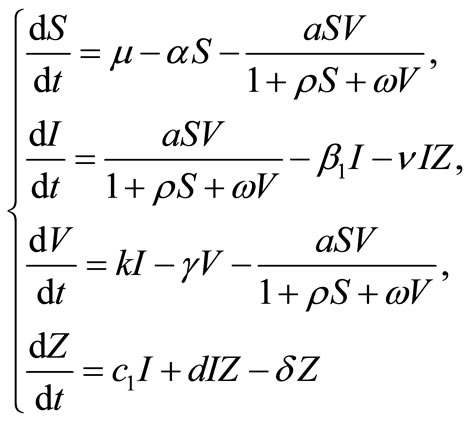 (1)
(1)
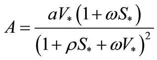
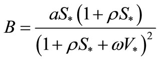
where, 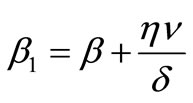 and
and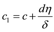 .
.
The constant , is the rate constant characterizing infection of the cells. The constants
  are positive.
In the above  and
and  represent the density of susceptible monocytes, infected monocytes, free virus particles and immune cells in 1 μl blood at time t, respective. The production of susceptible monocytes by bone marrow is assumed at a constant rate μ and the life span of susceptible monocytes is
 . The flow from susceptible monocytes to the infected monocytes depends on the incidence rate of susceptible monocytes and free virus particle. This rate is shown by
  where
where  is the incidence response of susceptible monocytes to free virus particles. The period of infected monocytes is assumed constant as
  . We assumed virus multiplication is at constant rate k and the virus clearance rate is at constant rate
 . We also assumed the immune cells are produced at constant rate
  and their life span is
 . Moreover we assumed there is stimulation of immune cells production due to the increase of infected cell which is proportional to the density infected monocytes at a constant rate c as well as from the contacts with infected cells at the rate d and the immune cells will eliminate the infected monocytes at a constant rate v. Finally, the positive constants
  and
and  have some biological meanings.
The above model is valid for only one serotype of dengue virus circulate in an infected host and dengue infects monocytes in blood stream.
For more detail the reader is referred to [4] and references therein.
The local stability of the equilibrium points of the system (1) for Lotka-Voltera functional response i.e.  , has been discussed in [4]. The model (1) is a generalization of the self-regulating cytotoxic T lymphocytes (CTL) response model. The predator-prey like CTL response model and the linear immune response model in chapter 6 of [5].
In this paper, we will analyze the global of stability of the viral free equilibrium for Beddington-DeAngelis incidence response,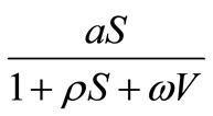 . In fact we will show that if this equilibrium is the only rest point of the system (1), then it is globally asymptotically stable. If there are some other equilibria, then the local stability of them depends on the values of the parameters.
2. Global Stability of the Uninfected Equilibrium
In this section, at first we will find the equilibrium points of the system (1) and the eigenvalues of this system at these points. This information leads us to prove the locally asymptotical stability of the equilibrium points.
At an equilibrium point of the system (1) we must have
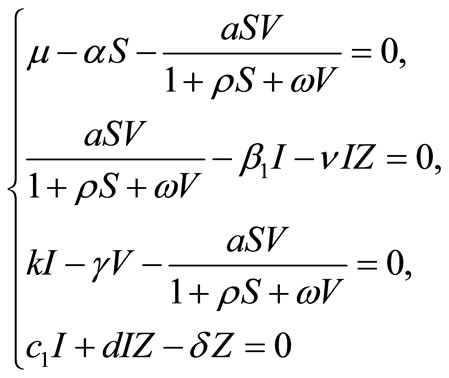 (2)
(2)
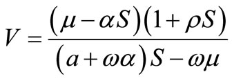
From the first equation we obtain,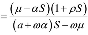 .
.
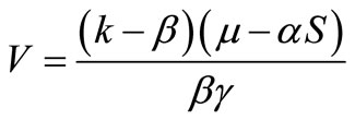
Substituting this value of V into the third equation yields, 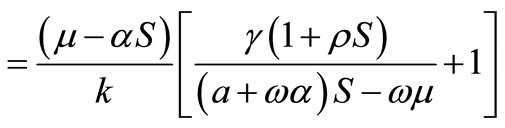 . From the fourth equation we obtain
  . Substituting these values of
  and
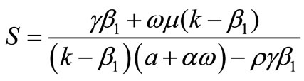
and  into the second equation yields,
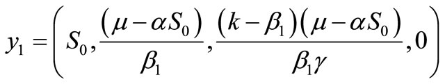
If,  , then from this, we have
 . Thus
 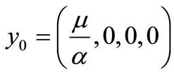 is one of the equilibrium points of the system (1). If,
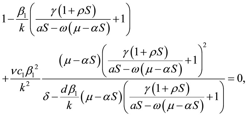
then
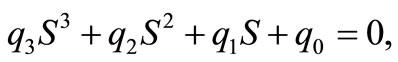 (3)
(3)
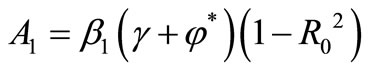
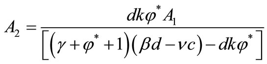
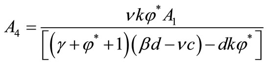
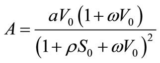
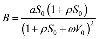
where,
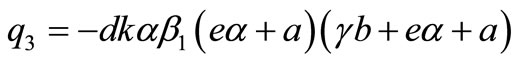 ,
,
and

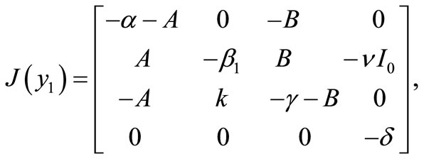
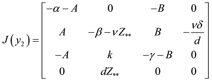
In the following we consider the stability property of the equilibrium point . In order to do this we check the sign of the eigenvalues of Jacobi matrix of (1) at
 . The Jacobi matrix is
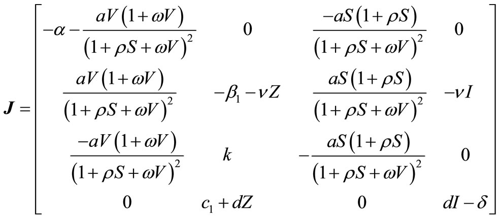 (4)
(4)
So the value of  at
at  is
is
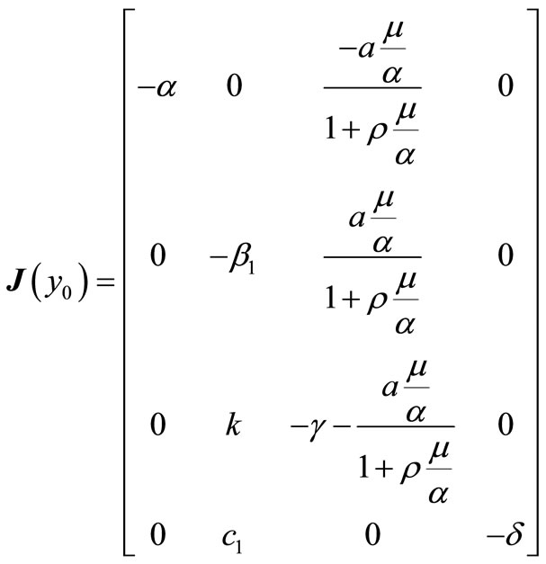
The eigenvalues of  are the roots of the characteristic polynomial
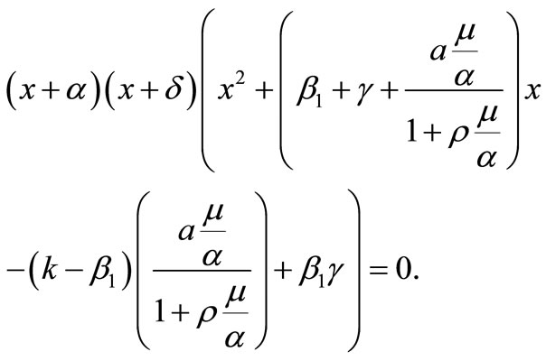
Thus,  and
and  are two of the eigenvalues and the other two are the roots of
 .
.
These roots are
where,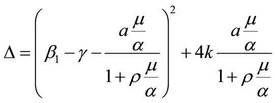 .
.
Clearly,  ,
,  and
and have negative real part. If
  has negative real part, then the equilibrium
  is locally asymptotically stable. But
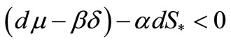
  is negative if and only if,
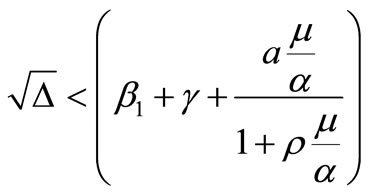 . This condition equals to,
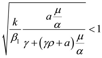 .
.
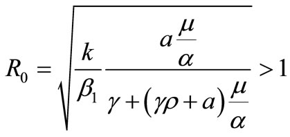
Set,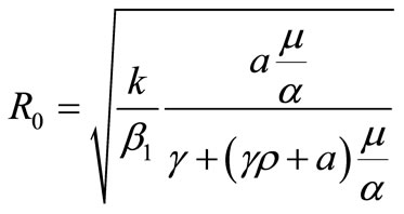 . This number is called the basic reproduction ratio [7].
Therefore we have the following theorem.
Theorem 2.1. If,  , the equilibrium point
  is locally asymptotically stable and if
 , the equilibrium
  is unstable.
Now we will show that if,  , then the equilibrium,
  is globally asymptotically stable. In order to see this, first of all consider the following domain in the
  space.
It follows that the flow generated by that system (1.1) gets into  on the boundary of
 . Let
. Let  for,
for,
 . Thus
  is a global attractor. Now in
  consider the following set for
 :
:
where, 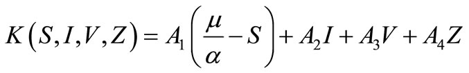
and

and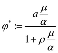 .
.
If we differentiate 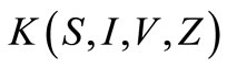 along the orbits of the system (1), we obtain:
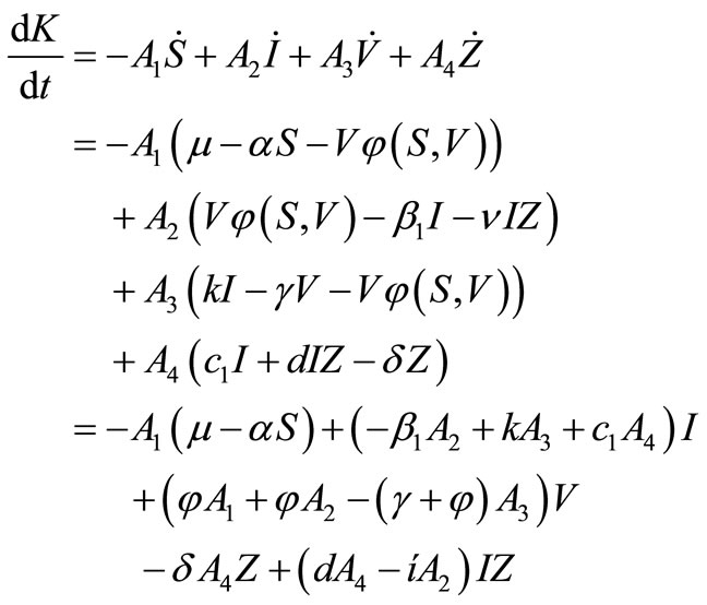
Here,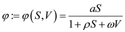 . Since on the surface
  of the boundary of
 , we have
  and
and  and
and  , therefore
 . Thus the flow gets into
  on,
on, . Hence the flow gets into
  from its boundary. Therefore
  is an attractor in D for all
 . But
. But . Thus
  is a global attractor. Thus we have proved the following theorem.
Theorem 2.2. If,  , then
  ,the uninfected equilibrium is the only equilibrium of the system (1). Moreover this equilibrium is globally asymptotically stable.
Since  is globally asymptotically stable for
 , any other equilibrium points of the system (1) cannot exist for
 . Therefore,
  is the unique equilibrium point for
 .
.
3. Stability of the Other Equilibrium Points
In this section, we consider the stability of the other rest point of the system (1). In order to this, we consider the Equation (3). First, we consider this equation for  and then for
 .
.
There are two cases for  as follows.
Case 1. 
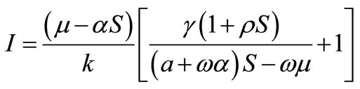
In this case, the system (1) has two equilibrium points,  and another one. To see this, from the first equation of (2) we obtain,
 . Since
from the fourth equation we get . Substituting these values of
  and
and  into the second equation yields,
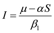 . By using the value of
  and the third equation we get
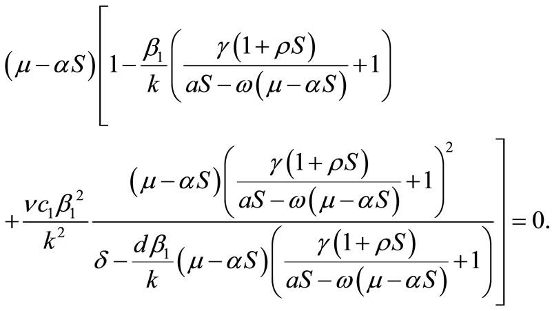
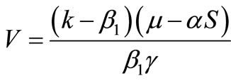 . Using these values into the equation (3), we obtain,
 .
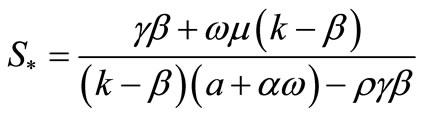
.
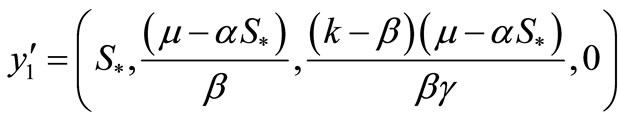
Therefore, we obtain
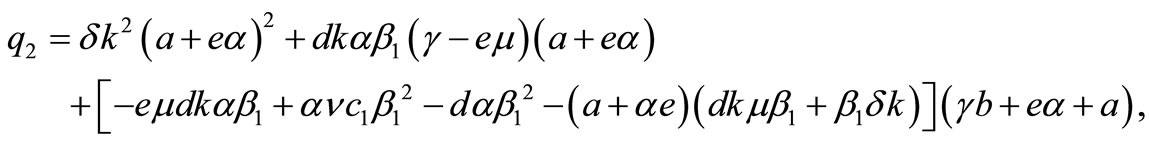
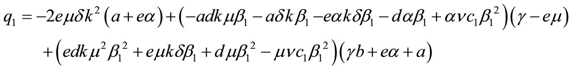
 where
where
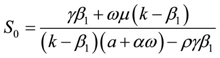 as the second rest point of the system (1).
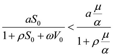
Notice that this rest point exists if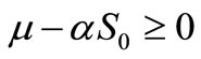 , or
, or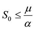 . If
. If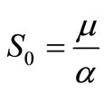 , this rest point is the same as
 . If
. If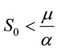 , then
 or
or
 .
.
Now, we consider the local stability of the equilibrium . By using the formula (4), the value of Jacobi matrix at
  is
is
where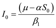 ,
,  ,
,
 and
and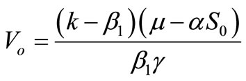 .
.
We calculate the eigenvalues of  as follow:
Thus one of the roots is . The other roots are given by

Here ,
,  and
and  .
.
By substituting the value of  and
and  in
in  and
and  we see that
  and
and  are positive. Moreover, it is easy to check that,
 . By the Rouths Hurwitz Criteria, all roots of the cubic polynomial have negative real part. Therefore we have the following theorem.
Theorem 3.1. If,  , then the equilibrium point
  exists and is locally asymptotically stable. Moreover the equilibrium
  exists and is unstable.
Remark 3.1. Since, the rest points and the eigenvalues depend continuously on the parameters, thus for small values of  and
and ,
,  exists and is locally asymptotically stable.
Case 2. 
In this case, the system (1) has three equilibrium points and  is one of them. Since
 , the fourth equation of the system (1) gives
  Therefore,
  or
or 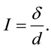 For
For , substituting the value of
  into the second equation yields,
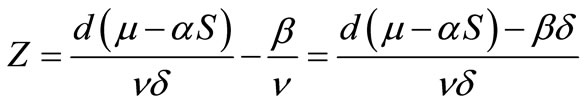
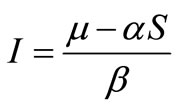 . By using the value of
  and the third equation we get,
 . Substituting values of
  and
and 
into the equation (3), we obtain,
 . Thus, we get
 as another rest point of the system (1).
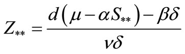
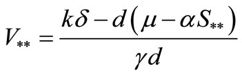
For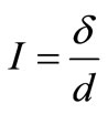 , by substituting this value of
  in the second equation of the system (1), we obtain
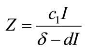
 . Then from the third equation we get,
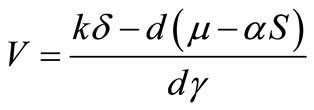 . By using this value of
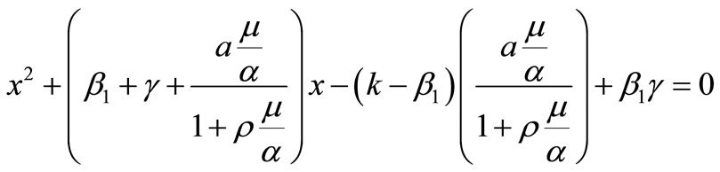
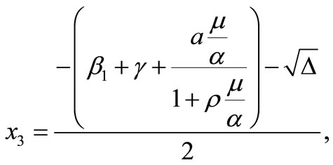
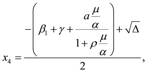
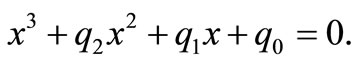
  into the first equation of the system (1), we obtain the following quadratic equation.
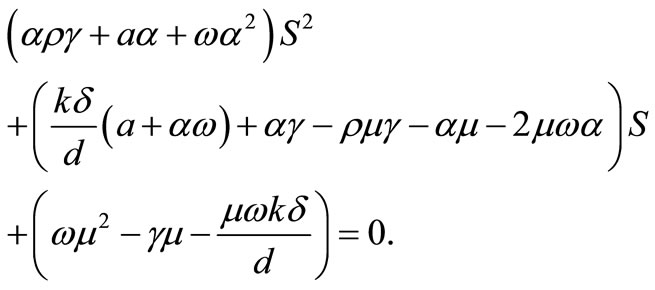
If 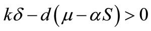 and
and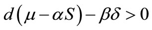 then
then 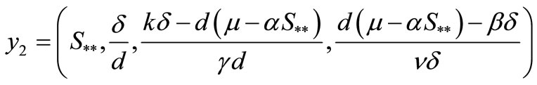
is another equilibrium point of the system (1) where  is the positive root of the above quadratic equation.
In the following, we consider the stability property of these points.
At first consider it for . Here we check the sign of the eigenvalues of Jacobi matrix of the system (1) at
 . From the formula (4) we have
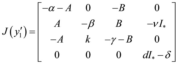
where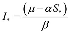 ,
,  ,
,
 and
and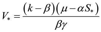 .
.
We calculate the eigenvalues of  as follows:
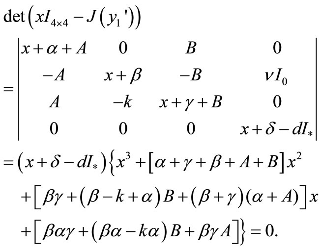
Thus one of the roots is . The other roots are given by
Here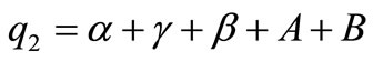 ,
,  and
and 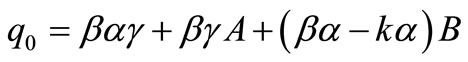 .
.
By substituting the value of  and
and  in
in  and
and  we will see that
  and
and  are positive. Moreover, it is easy to see that,
 . By the Rouths Hurwitz Criteria, all roots of the cubic polynomial have negative real part. If
 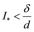 or
or
 , then real part of all of the eigenvalues are negative. Therefore the point
  is locally asymptotically stable.
Now we consider the stability property of the other equilibrium point, . From the formula (4) we have
 where
where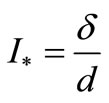 ,
,  ,
, 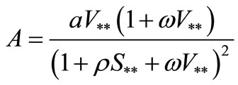 ,
,  and
and 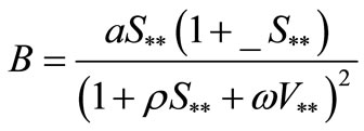 .
.
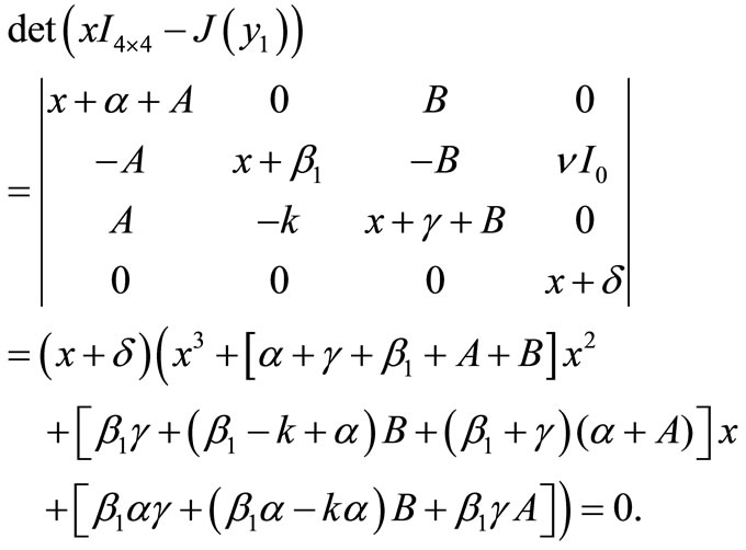
The eigenvalues of the matrix  are given by the algebraic equation,
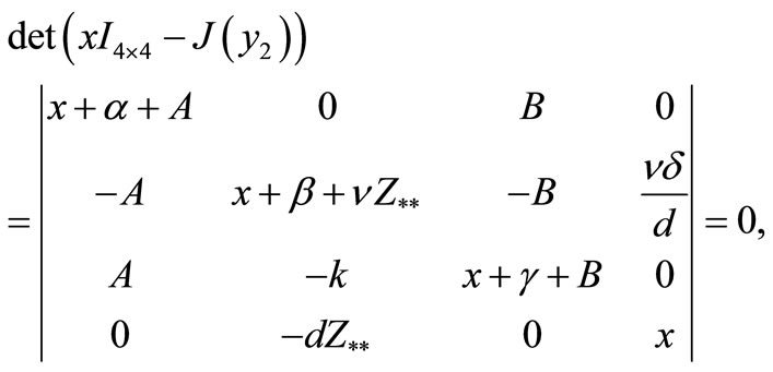
or
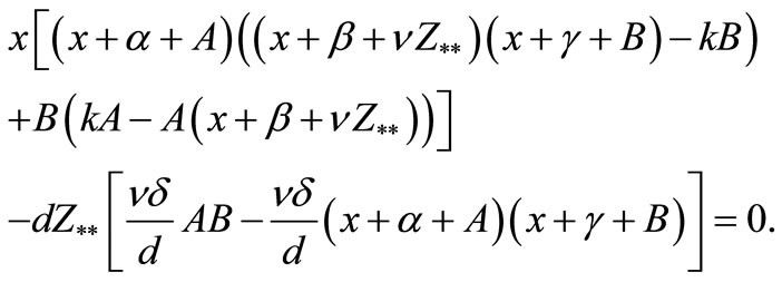
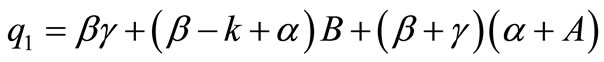
Then from the above equation we get
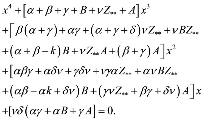
By considering the value of  it follows that all of the coefficients of the above equation are positive, then from Routh Hourwitz Criteria we see that all of the roots have negative real parts. Therefore we have the following theorem.
Theorem 3.2. For  and
and , we have the following results.
1) If , the equilibrium points
  and
and  are the only rest points of the system (1), then
  is unstable and
  is locally asymptotically stable.
2) If , then for
 , the equilibrium
 , is locally asymptotically stable and for
 , it becomes unstable. If
 ,
,
 and
and  are the only two rest points of the system (1) and
  does not exist.
3) If  and
and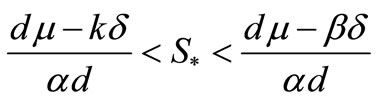 then the equilibrium
  exists and is locally asymptotically stable. Moreover the equilibrium points
  and
and  are unstable.
Remark 3.2. If , the point
  does not exist, therefore the point
  is the only endemic equilibrium point of the system (1). Also, for
and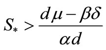 , the point
  is the only endemic equilibrium point.
Remark 3.3. 1) From continuous dependent of the equilibrium points and eigenvalues to the parameters, Theorem 3.1 and 3.2 must be valued for  and small.
2) For the case,  and large, if
 , the point
 is the unique equilibrium of the system
(1) which is globally asymptotically stable. If , the system (1) has a unique endemic equilibrium point,
  satisfying in the equations
 ,
,
 ,
,  and the equation (3). Here stability property of this point is not shown.
4. Numerical Simulation
For the following numerical simulations, we use parameters of T-cells as the parameters of immune cells, those are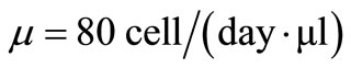 ,
,  days. The estimated value of
  is obtained by assuming that the equilibrium value of the density of immune cells in the absence of infection is 2000 cells.
In this model the endemic status of the disease depends on the individual response toward incoming viruses. The larger the invasion rate , the chance is higher to catch the disease. On the contrary the increase of the elimination rate
  of infected cell, the risk of infection is lower.
For ,
,
 ,
,
 , we have For
  we obtain the same result in the above table.
If  then for the same value of parameters we have the following table.
5. Conclusions
In order to understand the main characteristic of Dengue mystery, the author in [4] assumed that this virus can be eliminated by immune response which is described by the last equation of the system (1).
By using linear incidence rate of susceptible and free virus particle, they analyzed the existence of the endemic virus equilibria.
In this paper, from the analysis of the endemic equilibria it is found that, for Beddington DeAngelis incidence rate of susceptible and free virus particle, the same results are valid.
The reson for this correspondence is that in both models, the feature of the immune response is described by the term . However, the parameter
  in Beddington DeAngles makes the elimination of dengue virus by immune response in a shorter time. This fact can be seen by comparing Tables 1 and 2.
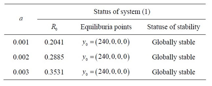
Table 1. status of equilibrium points of system (1) in the case .
.
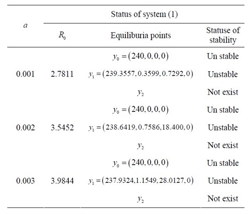
Table 2. status of equilibrium points of system (1) in the case ,
, .
.
By Theorem 2.2, if the basic reproduction number,  is less than one, then uninfected equilibrium point,
  is the only steady state point of system (1) and it is globally asymptotically state. This means that the virus is eliminated by immune response. For larger values of
  and
and ,
,  is more attractor and the virus is cleared much faster.
If the basic reproduction number,  is more than one; for
 , besides of the uninfected steady state
  which is uninfected, there are some infected steady state. Here we consider two cases of endemic virus.
Fist, for , we have only one infected endemic
 . If
. If , there is no immune response, so the density of susceptible moncytes equal zero. In
 , this density equals
 , so it does not depend on the other parameters for virus load of infected cell. For lager values of
  and
and , the infected endemic
  is closer to the uninfected endemic
  and it is more controllable.
Second, for  and
and , from Theorem 3.2 we see that if
  is negative or positive small, then there is only one infected endemic equilibrium
  which is stable. However if
  is positive and large, then the endemic virus equilibrium
  exists and is stable. This means that we found
  new threshold for
 . For condition
  is less than this threshold the dynamic of the model is qualitatively same as the case
 . When
  is greater than this threshold, we have a new endemic virus equilibrium,
  which is stable and the equilibrium points
  and
and  are unstable. From the components of the endemic equilibrium
  we see that after the onset of the symptom, if
  increases, the
  and
and  components of equilibria decrease and the
  and Z-components of equilibria will increase. Conversely, if
  and
and  increase, the
  and I-components of equilibria will decrease but the virus load increases at the initial viral infection.
For case  and large and
 , the model has a unique endemic virus. The
  and
and  components of this equilibrium point decrease as
  increases and the
  and Z-components of it increase as
  increases.
Therefore,  and
and  are the important parameters to capture the phenomena that dengue virus is quickly cleared in
  shorter time.
6. Acknowledgements
The authors would like to thank the anonymous reviewers for their valuable comments and suggestions to improve the manuscript.
REFERENCES
- WHO, “Tropical Disease Research, Making Health Research Work for Poor People,” Progress 2003-2004, World Health Organization, Geneva, 2005.
- D. J. Gubler, “Dengue and Dengue Hemorrhagic Fever,” Clinical Microbiology Reviews, Vol. 11, No. 3, 1998, pp. 480-496.
- E. A. Henchal and J. R. Putnak, “The Dengue Viruses,” Clinical Microbiology Reviews, Vol. 3, No. 4, 1990, pp. 376-396.
- N. Nuraini, H. Tasman, E. Soewono and K. A. Sidarto, “A With-In Host Dengue Infection Model with Immune Response,” Mathematical and Computer Modelling, Vol. 49, No. 5-6, 2009, pp. 1148-1155. doi:10.1016/j.mcm.2008.06.016
- M. A. Nowak and R. M. May, “Virus Dynamics: Mathematical Principles of Immunology and Viroloy,” Oxford University Press, Oxford, 2000.
- N. Bellomo, N. K. Li and P. Maini, “On the Foundation of Cancer Modeling: Selected Topics, Speculations and Perspectives,” Mathematical Models and Methods in Applied Sciences, Vol. 18 No. 4, 2008, pp. 593-646. doi:10.1142/S0218202508002796
- C. Castillo-Chavez, Z. Feng and W. Huang, “On the Computation of R0 and Its Role on Global Stability,” In: Mathematical Approaches for Emerging and Reemerging Infectious Diseases: An Introduction, Springer-Verlag, New York, 2002, pp. 229-250. doi:10.1007/978-1-4613-0065-6
- L. Esteva and C. Vargas, “Analysis of a Dengue Disease Transmission Model,” Mathematical Biosciences, Vol. 150, No. 2, 1998, pp. 131-151. doi:10.1016/S0025-5564(98)10003-2
- L. Esteva and C. Vargas, “A Model for Dengue Disease with Variable Human Population,” Journal of Mathematical Biology, Vol. 38, No. 3, 1999, pp. 220-240. doi:10.1007/s002850050147
- L. Esteva and C. Vargas, “Coexistence of Different Serotypes of Dengue Virus,” Journal of Mathematical Biology, Vol. 46, No. 1, 2003, pp. 31-47. doi:10.1007/s00285-002-0168-4
- Z. Feng and J. X. Velasco-Hernandez, “Competitive Exclusion in a Vector-Host Model for the Dengue Fever,” Journal of Mathematical Biology, Vol. 35, No. 5, 1997, pp. 523-544. doi:10.1007/s002850050064