Smart Grid and Renewable Energy
Vol.4 No.1(2013), Article ID:28135,12 pages DOI:10.4236/sgre.2013.41011
Hybrid Prediction Method for Solar Power Using Different Computational Intelligence Algorithms
![]()
Power Engineering Research Group (PERG), Central Queensland University, Rockhampton, Australia.
Email: m.hossain@cqu.edu.au
Received November 23rd, 2012; revised December 23rd, 2012; accepted December 30th, 2012
Keywords: Computational Intelligence; Heterogeneous Regressions Algorithms; Performance Evaluation; Hybrid Method; Mean Absolute Scaled Error (MASE).
ABSTRACT
Computational Intelligence (CI) holds the key to the development of smart grid to overcome the challenges of planning and optimization through accurate prediction of Renewable Energy Sources (RES). This paper presents an architectural framework for the construction of hybrid intelligent predictor for solar power. This research investigates the applicability of heterogeneous regression algorithms for 6 hour ahead solar power availability forecasting using historical data from Rockhampton, Australia. Real life solar radiation data is collected across six years with hourly resolution from 2005 to 2010. We observe that the hybrid prediction method is suitable for a reliable smart grid energy management. Prediction reliability of the proposed hybrid prediction method is carried out in terms of prediction error performance based on statistical and graphical methods. The experimental results show that the proposed hybrid method achieved acceptable prediction accuracy. This potential hybrid model is applicable as a local predictor for any proposed hybrid method in real life application for 6 hours in advance prediction to ensure constant solar power supply in the smart grid operation.
1. Introduction
Large scale penetration of solar power in the electricity grid provides numerous challenges to the grid operator, mainly due to the intermittency of sun. Since the power produced by a photovoltaic (PV) depends decisively on the unpredictability of the sun, unexpected variations of a PV output may increase operating costs for the electricity system as well as set potential threats to the reliability of electricity supply [1]. One of the main concerns of a grid operator is to predict changes of the solar power production, in order to schedule the reserve capacity and to administer the grid operations [2-6]. However, the prediction accuracy level of the existing methods for solar power prediction is not up to the mark; therefore, accurate solar power forecasting methods become very significant. Next to transmission system operators (TSOs), the prediction methods are required by various end-users as energy traders and energy service providers (ESPs), independent power producers (IPPs), etc. The accurate prediction methods are essential to provide inputs for different functions such as economic scheduling, energy trading and security assessment.
Many researches focus on providing a forecasting method in order to predict solar power production with expected accuracy. Depending on their input, these methods can be classified as physical or statistical approaches or jointly approach. The physical models use physical considerations, as meteorological (numerical weather predictions) and topological information, and technical characteristics of the PV (power curve, photo conversion efficiency and correction factor for photo conversion efficiency). Their intention is to get the most likely approximation of the local solar radiation and then use Model Output Statistics (MOS) to diminish the remaining error. Statistical models utilize descriptive variables and online measurements, typically employing recursive techniques, like recursive least squares or artificial neural networks. Moreover, physical models have to be used and statistical models may use Numerical Weather Prediction (NWP) models [7-11]. According to the literature review, an hourly irradiance producer [12] as well as based on a whole day [13] was invented by Gordon and Reddy. Knight et al. [14] demonstrated methods to generate irradiance data based on hour is known as GEN which involves the contribution of the month based standard irradiance data to produce hour based irradiance figures [14]. The hypothesis that simulations run with those produced data for a distinct one year time would provide fairly parallel outcomes to those gained from simulations determined by numerous years of calculated data was proved by Knight et al. [14]. Synthetically produced hourly varying solar radiation data and the temperature was employed as input data for the simulation program by Morgan [15].
To facilitate successful exploration for the best model, reliable techniques are required for combining different regression algorithms, creating ensembles, model testing etc. It is called meta-learning or ensemble learning research [16]. Since every inductive learning algorithm makes use of some biases, it performs well in some domains where its biases are suitable while it behaves poorly in other domains. One algorithm cannot be superior, in terms of generalization performance to another one among all the domains [17-18]. One approach to conquer this dilemma is to make a decision when a method may be appropriate for a given problem by selecting the best regression model according to cross validation [19]. A second, more accepted approach is to combine the capabilities of two or more regression methods [20]. To date, comparatively few researches have addressed ensembles for regression [20-22]. The success of the techniques that combine regression models comes from their ability to diminish the bias error as well as the variance error [23]. The bias is an assessment of how closely the model’s average prediction, measured over all possible training sets of fixed size. Variance is a measure of how the models’ predictions will differ from the average prediction of over all possible training sets of fixed size. Most of ensemble or hybrid methods described so far use models of one single class, e.g. neural networks [24] or regression trees [21] to predict renewable energy. Ensemble learning consists of two problems; ensemble generation: how the base models are generated and ensemble integration: how the base models’ predictions incorporated to get better performance. Ensemble generation can be differentiated as homogeneous if each base learning model employs the identical learning algorithm or heterogeneous if the base models can be developed from a variety of learning algorithms. There has been much empirical work on ensemble learning for regression in the perspective of neural networks, however there has been fewer research carried out in terms of using heterogeneous ensemble techniques to improve the performance.
In this paper, a novel hybrid method for solar power prediction is proposed that can be used to estimate PV solar power with improved prediction accuracy. Here, the term “hybridization” is anchored in the top most three selected heterogeneous regression algorithm based local predictors and a global predictor. The proposed method focuses on one of the two decisive problems of ensemble learning namely heterogeneous ensemble generation for solar power prediction. Figure 1 outlines the sequential structure of the proposed hybrid method of solar power prediction. For the time being this particular paper deals with the first two steps; presenting ensemble generation strategy and preliminary prediction performance of the local predictors based on the selected top most three regression algorithms.
Overview of the proposed hybrid prediction method is presented in Section 2. The data used in the experiment is described in Section 3. The experiment design for the ensemble generation, estimating and comparing the strengths of preliminary selected regression algorithms with 10 folds cross-validation and training and testing error estimator method are depicted in Section 4. Six hours ahead individual predictions performed by the initially selected regression algorithms and the accuracy of the prediction performances are validated with both the scale dependent and scale free error measurement metrics in Section 5. The detail theory about regression algorithms are presented in Section 6. Independent samples t-tests are carried out to evaluate the individual mean prediction performance of the preliminary selected regression algorithms as well as the pair wise comparisons for mean predicted values of those algorithms in Sections 7 and 8 respectively. Finally, the paper concludes with the concluding remarks and recommendations.
2. Description of the Hybrid Method for Solar Power Prediction
First of all, the ensemble generation is performed from a pool of regression algorithms. For this purpose the three top most regression algorithms to act as the local predictors are selected based on experimental results. Next, feature selection is carried out. The feature selection aspect is fairly significant for the reason that with the same training data it may happen that individual regression algorithm can perform better with different feature
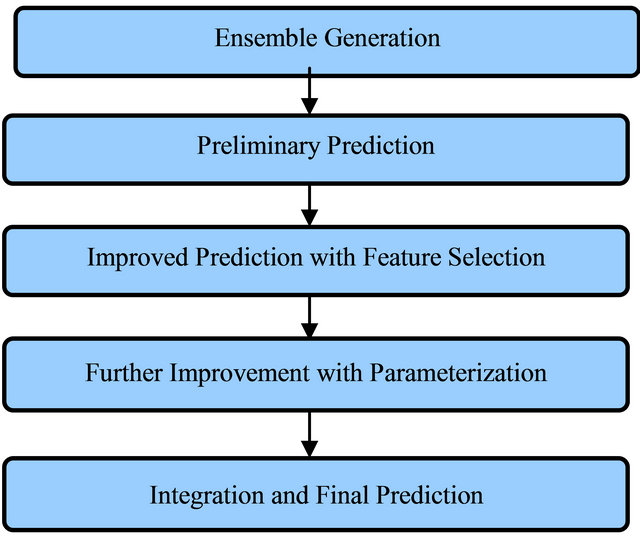
Figure 1. Outline of the proposed hybrid method.
sub sets [25]. The aim is to reduce the error of individual local predictors. The preliminary prediction using the selected three regression algorithms with feature selection is executed then. The structure of the proposed hybrid method for solar power prediction is shown in Figure 2 where  = Regression algorithm for local or base predictor.
In brief, the working mechanism of the proposed hybrid prediction method for solar power prediction can be stated in the following way. Raw set of data comprises stage one of data. Regression algorithm based local predictors operate in this stage. Stage two data are the preliminary predictions from the local predictors.
A further learning procedure takes place by means of
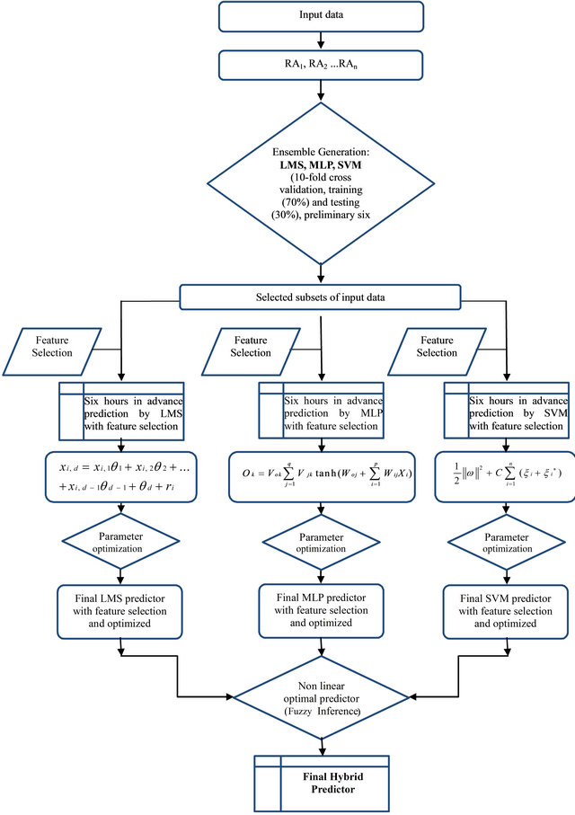
Figure 2. Structure of the hybrid method for solar power prediction.
placing level two data as input to produce the ultimate prediction. For this stage a regression algorithm is employed for finding out the way to integrate the outcomes from the foundation regression modules. One of the key conditions to successfully develop this hybrid prediction method is to collect recent, reliable, accurate and long term historical weather data of the particular location selected for the experiments. The following section continues with the description and analysis of the raw data used for this research.
3. Data Collection
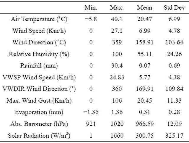
Historical solar data are a key element in solar power prediction systems. Rockhampton, a sub tropical city in Australia was chosen for the experiment of the proposed heterogeneous regression algorithms based hybrid method. The selected station is “Rockhampton Aero”, having latitude of −23.38 and longitude of 150.48. The recent data were collected from Commonwealth Scientific and Industrial Research Organization (CSIRO), Australia. In Figure 3 Renewable Energy Certificates (RECs) zones within Australia is shown where Rockhampton is identified within the most important zone [26]. Data was also collected from the Australian Bureau of Meteorology (BOM), the National Aeronautics and Space Administration (NASA), the National Oceanic and Atmospheric Administration (NOAA). Free data is available from National Renewable Energy Laboratory (NREL) and NASA. These are excellent for multi-year averages but perform poorly for hourly and daily measurements. After rigorous study the data provided by CSIRO was finally selected as the raw data is available in hourly resolution which is a significant aspect of the data set. Hourly raw data were gathered for a period of 2005 to 2010. Table 1 represents the attributes of the used data set as well as statistical properties of those attributes. The next sections will illustrate the procedure of base models generation i.e. ensemble generation.
4. Experiment Design
Ten popular regression algorithms namely Linear Regression (LR), Radial Basis Function (RBF), Support Vector Machine (SVM), Multilayer Perceptron (MLP), Pace Regression (PR), Simple Linear Regression (SLR), Least Median Square (LMS), Additive Regression (AR), Locally Weighted Learning (LWL) and IBK Regression have been used to find out ensemble generation. A unified platform is used with WEKA release 3.7.3 for all of the experiments. The WEKA is a Java based data mining tool [27] which is an efficient data pre-processing tool that encompasses a comprehensive set of learning algorithms with graphical user interface as well as command prompt. The accuracy of the model is justified by crossvalidation method and training-testing method.
4.1. K Fold Cross-Validation Error Estimator
Cross-validation, at times called rotation estimation is a method for assessing how the results of a statistical analysis will generalize to an independent data set. In  a data set
  is uniformly at random partitioned into
  folds of similar size
 . For the sake of clarity and without loss of generality; it is supposed that
 ![]() is multiple of
is multiple of . Let
. Let  be the complement data set of
 . Then, the algorithm
  induces a classifier from,
  and estimates its prediction error with
 . The
. The  prediction error estimator of
  is defined as follows [28]:
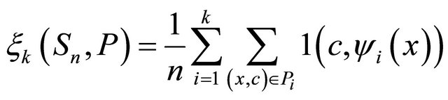 (1)
(1)
where  if
if  and zero otherwise. So, the
  error estimator is the average of the errors made by the classifiers
  in their respective divisions
 . The approximated error may be considered a random variable
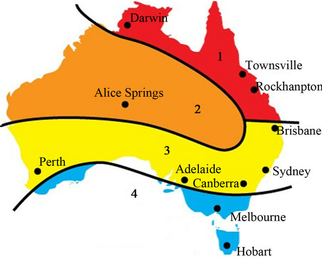
Figure 3. Renewable Energy Certificates (RECs) zones within Australia.
Table 1. Attributes of the raw data set and the corresponding statistics.
which relies on the training set Sn and the division . In Table 2 the results of applying 10 folds cross-validation method on initially selected regression algorithms are demonstrated. The above results clearly show that in terms of the mean absolute error (MAE) the most accurate one is the MLP regression algorithm. Next to the MLP, SVM is in the second best position and LMS regression algorithm is in the third best position.
4.2. Training and Testing Error Estimator
In this error estimator method, a common rule of thumb is to use 70% of the data set for training and 30% for testing. In Table 3 the results of applying training and testing error estimator method on initially selected regression algorithms are illustrated.
Based on the experimental outcome the MLP is the number one choice, SVM is in the second best position and LMS regression algorithm is in the third best position. Both of the 10 folds cross-validation and training and testing method suggests the top most three algori-
Table 2. Results of applying 10 folds cross validation method on the data set.
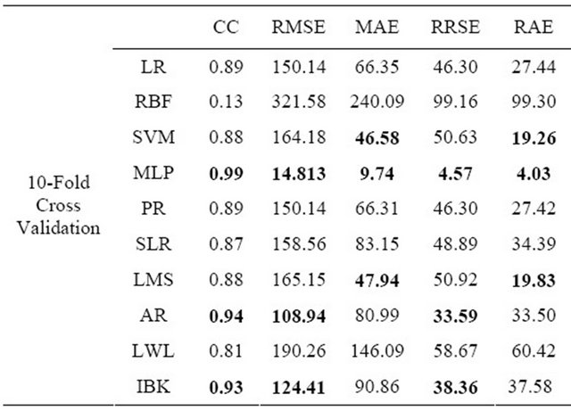
Table 3. Results of applying training and testing method on the data set.
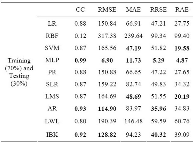
thms for this task are MLP, SVM and LMS in descending order. Next, six hours ahead individual predictions performed by the initially selected regression algorithms and the accuracy of the prediction performances are validated with both the scale dependent and scale free error measurement metrics.
5. Using Preliminary Short Term Prediction with Base Regression Algorithms
The six hours ahead solar radiation prediction with the potential regression algorithms were performed to compare the errors of the individual prediction to select three decisive regression algorithms for the ensemble generation. In Table 4, the summary of six hours in advance prediction error for different regression algorithms with both the scale dependent and scale free prediction accuracy validation metrics are presented.
Prediction Accuracy Validation Metrics
In general, there are four types of prediction-error metrics [29]. Those are: scale dependent metrics as for example MAE; metrics related to percentage of error such as mean absolute percentage error (MAPE); metrics regarding relative error which computes the ratio of error between a selected and a novel approach; and finally scale free error measurements that is not dependent to scale of the data and can be used to compare forecast systems on a distinct series and also to compare forecast accuracy between series such as MASE.
From the individual prediction results the regression algorithms are ranked. According to [30], MAE is strongly suggested for error measurement. Hence, the ranking is done based on the MAE of those regression algorithms’ predictions.
Accuracy of the preliminary experimental results of distinct base predictor was also analyzed according to MASE [29]. MASE is scale free, less sensitive to outlier; and less variable to small samples. MASE is suitable for uncertain demand series as it never produces infinite or
Table 4. Six hours ahead prediction errors of different regression algorithms.
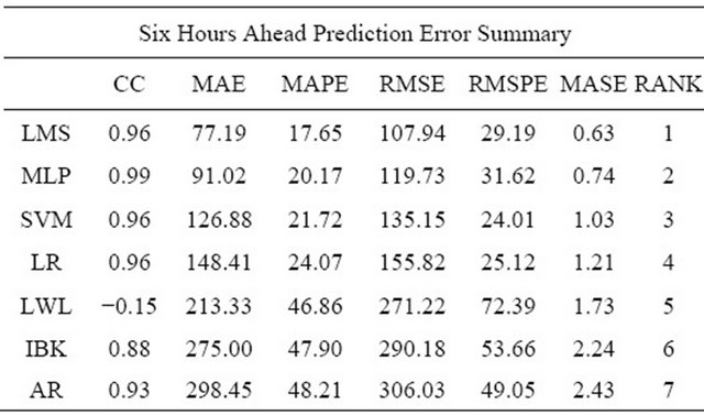
undefined results. It indicates that the forecast with the smallest MASE would be counted the most accurate among all other alternatives [29]. Equation (2) states the formula to calculate MASE.
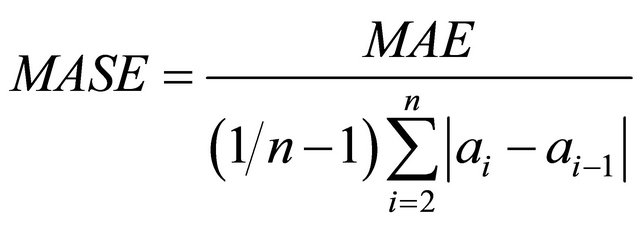 (2)
(2)
 (3)
(3)
In Equations (2) and (3), ![]() = number of instances,
= number of instances,  = actual values and
  = predicted outputs. In Figure 4 the prediction performance of the preliminary selected regression algorithms in terms of various error validation metrics used are portrayed.
Based on MAE and MASE the top most three regression algorithms for ensemble generation are LMS, MLP and SVM. In Figures 5-7 the comparison between the actual and predicted values of these three regression algorithms are graphically presented respectively.
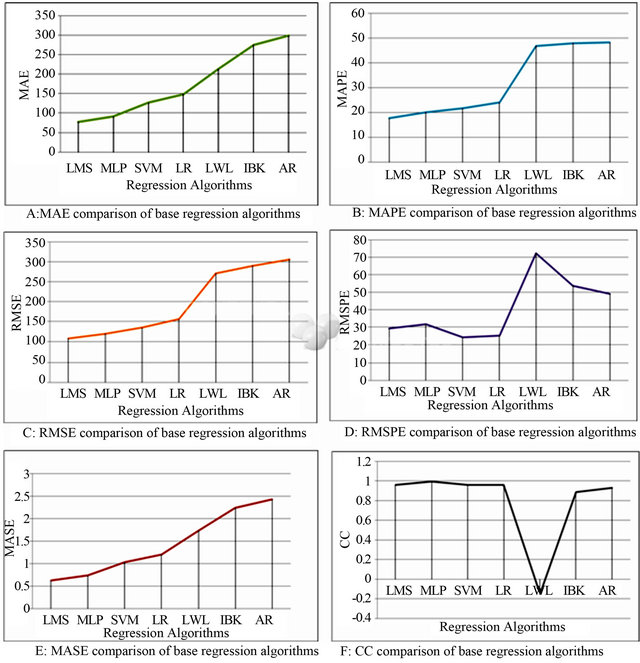
Figure 4. Prediction performance of the regression algorithms with A: MAE, B: MAPE, C: RMSE, D: RMSPE, E: MASE and F: CC error validation metrics.
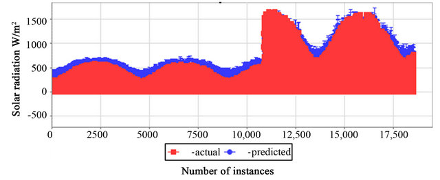
Figure 5. Prediction performance of the LMS regression algorithm.
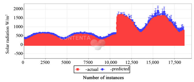
Figure 6. Prediction performance of the MLP regression algorithm.
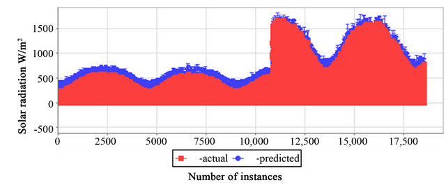
Figure 7. Prediction performance of the SVM regression algorithm.
6. Selected Regression Algorithms for Ensemble Generation
6.1. Support Vector Machine (SVM)
The Support Vector (SV) algorithm is a nonlinear generalization of the “Generalized Portrait” algorithm developed in Russia in the sixties [31]. One of the artificial intelligence based renewable energy forecasting methods described in the literature [32,33], which involves the socalled Support Vector Machines. Such models are less rigid in terms of architecture than Artificial Neural Networks (ANNs) and may allow one to save even more modeling efforts when designing prediction models. While other statistical models are estimated following the empirical risk minimization principle, i.e. the minimization of loss function over the learning set and the checking of the generalization ability with some criteria, the SVM theory is based on the structural risk minimization principle, which consists on directly minimizing an upper bound on the generalization error, and thus on future points [34]. There is today a large interest in applying SVMs for several purposes including renewable energy forecasting [35-39].
6.2. Least Median Square (LMS)
Strong and fast regression methods are necessary that are able to cope with the various challenges involved in the successful implementation of smart grid. LMS is one of the potential factors which can be used to serve the purpose of the successful implementation of smart grid [40].
The least median square is basically consists of adjusting the parameters of a model function to best fit a data set. Rousseeuw’s LMS linear regression estimator [41] is amongst the best known and most extensively used robust estimators. The LMS estimator is defined formally as follows. Consider a set  of
of ![]() points in
points in , where
 . A parameter vector
  that best fits the data by the linear model is likely to be computed.
 (4)
(4)
for all  where
where  are the (unknown) errors, or residuals.
6.3. Multilayer Perception (MLP)
MLP which is one of the types of ANNs have been used in diverse applications as well as in renewable energy problems. ANNs have been used by various authors in the field of solar energy; for modeling and design of a solar steam generating plant, for the estimation of a parabolic trough collector intercept factor and local concentration ratio and for the modeling and performance prediction of solar water heating systems. They have also been used for the estimation of heating loads of buildings, for the prediction of air flow in a naturally ventilated test room and for the prediction of the energy consumption of a passive solar building [42].
In all those models multiple hidden layer architecture has been used. Errors reported in these models are well within acceptable limits, which clearly suggest that ANNs can be used for modeling in other fields of renewable energy production and use. Research works using ANNs in the field of renewable energy as well as in other energy systems are found in the literature review. This includes the use of ANNs in solar radiation and wind speed prediction, photovoltaic systems, building services systems and load forecasting and prediction [42].
In general MLP can have numerous hidden layers (Figure 8), however according to Hornik; a neural network with single hidden layer is capable to estimate a function of any complexity [43]. If a MLP with one hidden layer is considered, tanh as an activation function and a linear output unit, the equation unfolding the network structure can be expressed as:
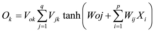 (5)
(5)
where  is the output of the
  output unit,
  and
and  are the network weights,
 ![]() is the number of network inputs, and
is the number of network inputs, and  is the number of hidden units. Throughout the training progression, weights are altered in such a way that the difference between the obtained outputs
  and the desired outputs
  is minimized, which is typically done by minimizing the following error function:
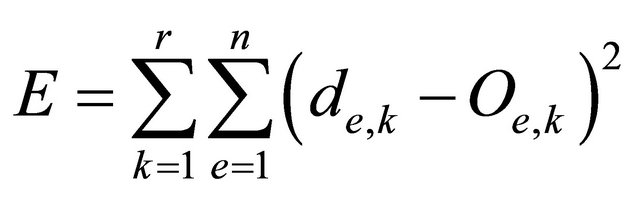 (6)
(6)
where  is the number of network outputs and
 ![]() is the number of training examples. The minimization of the error function is usually done by gradient descent methods, which have been comprehensively investigated in the field of optimization theory [44].
is the number of training examples. The minimization of the error function is usually done by gradient descent methods, which have been comprehensively investigated in the field of optimization theory [44].
7. Statistical Test
T-test is employed to verify the algorithm accuracy performances in the experiments. In this paper the independent samples T-Tests are carried out in order to justify whether any significant difference exists between the actual and predicted values achieved by the selected three regression algorithms. These tests are done in order ensure the potentiality of those selected heterogeneous regression algorithms for the suggested hybrid method. The t-test is executed with the SPSS package-PASW Statistics 18.
7.1. T-Test to Compare the Mean Actual and Predicted Values of LMS
For the least median square (LMS) regression algorithm, an equal variances  test failed to reveal a statistically reliable difference between the mean number of the actual and predicted values of solar radiation with actual
 ,
, and predicted data (
 ,
, ),
), 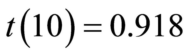 , two tailed significance value
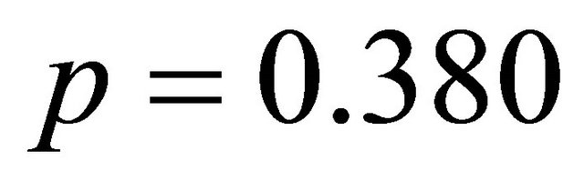 , significance level
 . The decision rule is given by: if
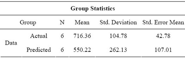
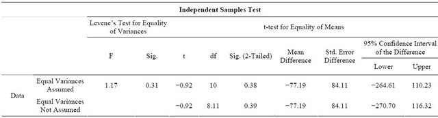
 , then reject the obtained result. In this instance, 0.380 is not less than or equal to 0.05 and fail to reject the obtained result. That implies that the test failed to observe any significant difference between the actual and predicted values performed by LMS on average. In Table 5 the group statistics with Mean (M), Standard Deviation (S) and Standard Error Mean for the actual and predicted values of LMS is represented. In Table 6 the independent samples t-test results for the actual and predicted values of LMS is illustrated.
In the same way t-test to compare the mean actual and predicted values of MLP and t-test to compare the
Table 5. Group statistics of LMS.
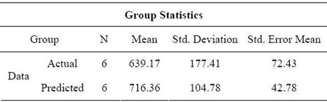
Table 6. Independent samples t-test results for LMS.
actual and predicted values of SVM are performed and the corresponding results are discussed in the results and discussions section of this paper.
Observing all the above mentioned results, it is failed to observe any significant difference between the actual and predicted values performed by LMS regression algorithm on average. Therefore, the test failed to reject the obtained result for LMS regression algorithm.
7.2. T-Test to Compare the Mean Predicted Values between LMS and MLP
For the LMS and MLP regression algorithm, an equal variances t test failed to reveal a statistically reliable difference between the mean number of predicted values of solar radiation with LMS ( ,
, ) and MLP (
 ),
),  two tailed significance value
 , significance level
 . The decision rule is given by: if
 , then reject the obtained result. In this instance, 0.180 is not less than or equal to 0.05 and fail to reject the obtained result. That implies that the test failed to observe any significant difference between the predicted values performed by the pair LMS: MLP on average. In Table 7 the group statistics with M, s and Standard Error Mean for the predicted values of LMS: MLP is represented.
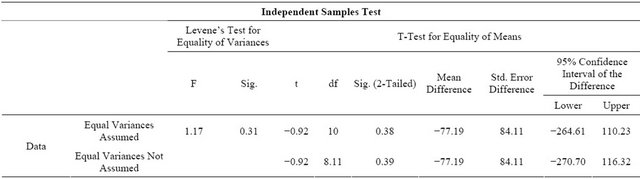
In Table 8 the independent samples t-test results for the predicted values of LMS: MLP is illustrated. In the same way t-test to compare the mean predicted values between LMS and SVM and t-test to compare the predicted values between MLP and SVM are performed and the corresponding results are discussed in the results and discussions section of this paper. All the above mentioned results in Table 8 failed to observe any significant
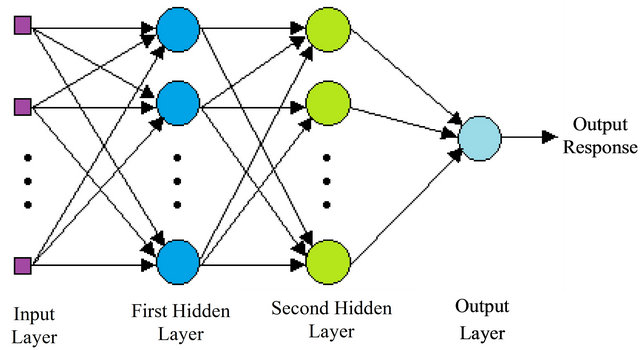
Figure 8. Architecture of a MLP with two hidden layers.
Table 7. Group statistics of the pair LMS and MLP.
difference between the predicted values performed by the pair LMS: MLP on average. Therefore, the test failed to reject the obtained results for the pair LMS: MLP regression algorithm.
8. Results and Discussions
The ensemble generation through empirically selected heterogeneous regression algorithms are presented in this paper. Those potential regression algorithms were applied as local predictors of the proposed hybrid method for six hour in advance prediction of solar power. Several performance criteria found in the solar power prediction method literature as: the training time, the modeling time and the prediction error. As the training process was in offline mode, the first two criteria were not considered to be relevant for this paper. In this context, the prediction performance was evaluated only in term of prediction error, defined as the difference between the actual and the forecasted values and based on statistical and graphical approaches. T-tests were performed as statistical error test criteria. For the individual performance of LMS, MLP and SVM regression algorithm, an equal variances t-test failed to reveal a statistically reliable difference between the mean number of actual and predicted values of solar radiation with actual and predicted data. In Table 5 the group statistics with M, s and Standard Error Mean for LMS was presented. In Table 6 the independent samples t-test results for LMS was illustrated. To compare the mean predicted values between the LMS: MLP, LMS: SVM and MLP: SVM regression algorithm, an equal variances t test failed to reveal a statistically reliable difference between the mean number of predicted values of solar radiation with LMS and MLP; with MLP and SVM. But for the instance of the pair LMS: SVM trivial difference between the predicted values is observed. Therefore, the obtained result is rejected. But this inconsistency can be eliminated by the proper selection of the kernel function and the optimal parameters of SVM for this purpose. In Table 7 the group statistics with M, s and Standard Error Mean for the predicted values of LMS: MLP was represented. In Table 8 the independent samples t-test results for the mean predicted values of LMS: MLP was illustrated. All the results found from the t-tests clearly indicate that the heterogeneous regression algorithms selected for the suggested hybrid method are more accurate and prospective. In Figure 5, the prediction performance of the preliminary selected regression algorithms in terms of various error validation metrics used are presented graphically. While the 2-D error prediction form (Figures 5-7) for the three proposed regression algorithm based predictors were presented as graphical error performance. In Table 4, referring to the MAE and MASE criteria, it is observed that LMS, MLP and SVM have the lowest prediction error. Therefore, these three
Table 8. Independent samples t-test results for the pair LMS and MLP.
regression algorithms are empirically proved to be potential for the proposed hybrid prediction method.
9. Conclusion
In this paper, based on heterogeneous regression algorithms a novel hybrid method for solar power prediction that can be used to estimate PV solar power with improved prediction accuracy is presented. The hybridization aspect is anchored in the top most selected heterogeneous regression algorithm based local predictors as well as a global predictor. One of the two decisive problems of ensemble learning namely heterogeneous ensemble generation for solar power prediction is mainly focused in this research. There are scopes to further improve the prediction accuracy of the selected individual regression algorithms namely LMS, MLP and SVM. As a consequence, the next step will be the efficient utilization of the feature selection aspect on the used data set to reduce the generalized error of those regression algorithms. Further tuning can be achieved through the parameter restructuring of those regression algorithms to make them as accurate and diverse as possible as well as to formulate the proposed hybrid method more effective. Finally, another regression algorithm or learning algorithm will be found out empirically to nonlinearly combine or integrate the individual predictions supplied from the improved local predictors. Further application of the proposed ensemble will include distributed intelligent management system for the cost optimization of a smart grid.
REFERENCES
- B. Parsons, M. Milligan, B. Zavadil, D. Brooks, B. Kirby, K. Dragoon and J. Caldwell, “Grid Impacts of Wind Power: A Summary of Recent Studies in the United States,” National Renewable Energy Laboratory, Madrid, 2003.
- R. Doherty and M. O’Malley, “Quantifying Reserve Demands Due to Increasing Wind Power Penetration,” 2003 IEEE Bologna Power Tech Conference Proceedings, Bologna, Vol. 2, 23-26 June 2003, pp. 23-26.
- R. Doherty and M. O’Malley, “A New Approach to Quantify Reserve Demand in Systems with Significant Installed Wind Capacity,” IEEE Transactions on Power Systems, Vol. 20, No. 2, 2005, pp. 587-595. doi:10.1109/TPWRS.2005.846206
- N. Hatziargyriou, A. Tsikalakis, A. Dimeas, D. Georgiadis, A. Gigantidou, J. Stefanakis and E. Thalassinakis, “Se- curity and Economic Impacts of High Wind Power Penetration in Island Systems,” Proceedings of Cigre Session, Paris, 30 August-3 September 2004, pp. 1-9.
- N. Hatziargyriou, G. Contaxis, M. Matos, J. A. P. Lopes, G. Kariniotakis, D. Mayer, J. Halliday, G. Dutton, P. Dokopoulos, A. Bakirtzis, J. Stefanakis, A. Gigantidou, P. O’Donnell, D. McCoy, M. J. Fernandes, J. M. S. Cotrim and A. P. Figueira, “Energy Management and Control of Island Power Systems with Increased Penetration from Renewable Sources,” Power Engineering Society Winter Meeting, Vol. 1, No. 27-31, 2002, pp. 335-339.
- E. D. Castronuovo and J. A. P. Lopes, “On the Optimization of the Daily Operation of a Wind-Hydro Power Plant,” IEEE Transactions on Power Systems, Vol. 19, No. 3, 2004, pp. 1599-1606. doi:10.1109/TPWRS.2004.831707
- M. C. Alexiadis, P. S. Dokopoulos, and H. S. Sahsamanoglou, “Wind Speed and Power Forecasting Based on Spatial Correlation Models,” IEEE Transactions on Energy Conversion, Vol. 14, No. 3, 1999, pp. 836-842. doi:10.1109/60.790962
- T. G. Barbounis, J. B. Theocharis, M. C. Alexiadis and P. S. Dokopoulos, “Long-Term Wind Speed and Power Forecasting Using Local Recurrent Neural Network Models,” IEEE Transactions on Energy Conversion, Vol. 21, No. 1, 2006, pp. 273-284. doi:10.1109/TEC.2005.847954
- L. Landberg, G. Giebel, H. A. Nielsen, T. Nielsen and H. Madsen, “Short-Term Prediction—An Overview,” Wind Energy, Vol. 6, No. 3, 2003, pp. 273-280. doi:10.1002/we.96
- G. Giebel, L. Landberg, G. Kariniotakis and R. Brownsword, “State-of-the-Art on Methods and Software Tools for Short-Term Prediction of Wind Energy Production,” EWEC, Madrid, 16-19 June 2003, pp. 27-36.
- G. Giebel, R. Brownsword and G. Kariniotakis, “The State of the Art in Short-Term Prediction of Wind Power: A Literature Overview,” 2003. http://130.226.56.153/rispubl/vea/veapdf/ANEMOS_giebel.pdf
- J. M. Gordon and T. A. Reddy, “Time Series Analysis of Hourly Global Horizontal Solar Radiation,” Solar Energy, Vol. 41, No. 5, 1988, pp. 423-429.
- J. M. Gordon and T. A. Reddy, “Time Series Analysis of Daily Horizontal Solar Radiation,” Solar Energy, Vol. 41, No. 3, 1988, pp. 215-226. doi:10.1016/0038-092X(88)90139-9
- K. M. Knight, S. A. Klein and J. A. Duffie, “A Methodology for the Synthesis of Hourly Weather Data,” Solar Energy, Vol. 46, No. 2, 1991, pp. 109-120. doi:10.1016/0038-092X(91)90023-P
- T. R. Morgan, “The Performance and Optimization of Autonomous Renewable Energy Systems,” Ph.D. Thesis, University of Wales, Cardiff, 1996.
- N. Jankowski, K. Grąbczewski and W. Duch, “Hybrid Systems, Ensembles and Meta-Learning Algorithms,” 2008. http://www.is.umk.pl/WCCI-HSEMLA/
- S. B. Kotsiantis and P. E. Pintelas, “Predicting Students’ Marks in Hellenic Open University,” Proceedings of 5th IEEE International Conference on Advanced Learning Technologies, Kaohsiung, 5-8 July 2005, pp. 664-668.
- S. Kotsiantis, G. Tsekouras, C. Raptis and P. Pintelas, “Modelling the Organoleptic Properties of Matured Wine Distillates,” MLDM’05 Proceedings of the 4th International Conference on Machine Learning and Data Mining in Pattern Recognition, Vol. 3587, 2005, pp. 667-673.
- A. Sharkey, N. Sharkey, U. Gerecke and G. Chandroth, “The Test and Select Approach to Ensemble Combination,” Springer-Verlag, Cagliari, 2000.
- N. L. Hjort and G. Claeskens, “Frequentist Model Average Estimators,” Journal of the American Statistical Association, Vol. 98, No. 464, 2003, pp. 879-899. doi:10.1198/016214503000000828
- L. Breiman, “Bagging Predictors,” Machine Learning, Vol. 24, No. 2, 1996, pp. 123-140. doi:10.1007/BF00058655
- R. Zemel and T. Pitassi, “A Gradient-Based Boosting Algorithm for Regression Problems,” MIT Press, Cambridge, 2001.
- G. Brown, J. Wyatt and P. Tino, “Managing Diversity in Regression Ensembles,” Journal of Machine Learning Research, Vol. 6, No. 1, 2005, pp. 1621-1650.
- U. Naftaly, N. Intrator and D. Horn, “Optimal Ensemble Averaging of Neural Networks,” Network, Vol. 8, No. 3, 1997, pp. 283-296. doi:10.1088/0954-898X/8/3/004
- P. Langley, “Selection of Relevant Features in Machine Learning,” AAAI Press, New Orleans, 1994.
- J. Harburn, “RECs/STCs-What Are They and How Are They Calculated?” http://www.solarchoice.net.au/blog/recs-what-are-they-and-how-are-they-calculated/
- R. Remco, Bouckaert, E. Frank, M. Hall, R. Kirkby, P. Reutemann, A. Seewald and D. Scuse, “WEKA Manual for Version 3-7-3,” The University of Waikato, New Zealand, 2010.
- S. Shevade, S. Keerthi, C. Bhattacharyya and K. Murthy, “Improvements to the SMO Algorithm for SVM Regression,” IEEE Transactions on Neural Networks, Vol. 11, No. 5, 2000, pp. 1188-1183. doi:10.1109/72.870050
- R. J. Hyndman and A. B. Koehler, “Another Look at Mea- sures of Forecast Accuracy,” International Journal of Forecasting, Vol. 22, No. 4, 2005, pp. 679-688.
- C. J. Willmott and K. Matsuura, “Advantages of the Mean Absolute Error (MAE) over the Root Mean Square Error (RMSE) in Assessing Average Model Performance,” Climate Research, Vol. 30, No. 1, 2005, pp. 79-82. doi:10.3354/cr030079
- V. Vapnik and A. Lerner, “Pattern Recognition Using Generalized Portrait Method,” Automation and Remote Control, Vol. 24, No. 6, 1963, pp. 774-780.
- K. Larson and T. Gneiting, “Advanced Short-Range Wind Energy Forecasting Technologies-Challenges, Solutions and Validation,” CD-Proceedings of the Global Wind Power Conference, Chicago, 28-31 March 2004, pp. 67-73.
- D. Monn, D. Christenson and R. Chevallaz-Perrier, “Support Vector Machines Technology Coupled with Physics-Based Modeling for Wind Facility Power Production Forecasting,” CD-Proceedings of the Global Wind Power Conference, Chicago, 28-31 March 2004, pp. 97-102.
- G. Kariniotakis, “Estimation of the Uncertainty in Wind Power Forecasting,” Ph.D. Thesis, Department of Energy, Ecole des Mines de Paris, Paris, 2006.
- M. Mohandes, T. Halawani and R. A. Hussain, “Support Vector Machines for Wind Speed Prediction,” Renewable Energy, Vol. 29, No. 6, 2004, pp. 939-947. doi:10.1016/j.renene.2003.11.009
- J. Zeng and W. Qiao, “Support Vector Machine-Based Short-Term Wind Power Forecasting,” Proceedings of the IEEE PES Power System Conference and Exposition, Arizona, 20-23 March 2011, pp. 1-8.
- J. Shi, W. Lee, Y. Liu, Y. Yang and P. Wang, “Forecasting Power Output of Photovoltaic System Based on Weather Classification and Support Vector Machine,” IEEE Industry Applications Society Annual Meeting (IAS), Orlando, 9-13 October 2011, pp. 1-6.
- N. Sharma, P. Sharma, D. Irwin and P. Shenoy, “Predicting Solar Generation from Weather Forecasts Using Machine Learning,” Proceedings of the 2nd IEEE International Conference on Smart Grid Communications, Brussels, 17-20 October 2011, pp. 32-37.
- K. R. Müller, A. Smola, G. Rätsch, B. Schölkopf, J. Kohlmorgen and V. Vapnik, “Using Support Vector Machines for Time Series Prediction,” In: B. Schölkopf, C. Burges and A. Smola, Eds., Advances in Kernel Methods—Support Vector Learning, MIT Press, Cambridge, 1998.
- O. Kramer, B. Satzger and J. Lässig, “Power Prediction in Smart Grids with Evolutionary Local Kernel Regression,” International Computer Science Institute, Berkeley. http://www.icsi.berkeley.edu/pubs/algorithms/powerprediction10.pdf
- P. J. Rousseeuw, “Least Median of Squares Regression,” Journal of American Statistics, Vol. 79, No. 388, 1984, pp. 871-880. doi:10.1080/01621459.1984.10477105
- S. A. Kalogirou, “Artificial Neural Networks in Renewable Energy Systems Applications: A Review,” Renewable and Sustainable Energy Reviews, Vol. 5, No. 4, 2001, pp. 373-401.
- K. M. Hornik, M. Stinchcombe and H. White, “Multilayer Feed Forward Networks Are Universal Approximator,” Neural Networks, Vol. 2, No. 2, 1989, pp. 359-366. doi:10.1016/0893-6080(89)90020-8
- R. Fletcher, “Practical Methods of Optimization,” 2nd Edition, Wiley, Chichester, 1990.