Smart Grid and Renewable Energy
Vol.3 No.4(2012), Article ID:24733,10 pages DOI:10.4236/sgre.2012.34045
FEDRP Based Model Implementation of Intelligent Energy Management Scheme for a Residential Community in Smart Grids Network
![]()
1Electrical Engineering Department, NWFP University of Engineering and Technology, Peshawar, Pakistan; 2Electrical Engineering Department, COMSATS Institute of Information Technology, Abbottabad, Pakistan; 3Electrical Engineering Department, Gandhara Institute of Science and Technology, Peshawar, Pakistan; 4IT Department, Hazara University, Havalian, Pakistan.
Email: hallianali@ciit.net.pk
Received June 29th, 2012; revised July 29th, 2012; accepted August 6th, 2012
Keywords: Demand Response (DR); FEDRP; Intelligent Energy Management (IEM); Residential Area Networks (RAN); Smart Grids
ABSTRACT
In the framework of liberalized deregulated electricity market, dynamic competitive environment exists between wholesale and retail dealers for energy supplying and management. Smart Grids topology in form of energy management has forced power supplying agencies to become globally competitive. Demand Response (DR) Programs in context with smart energy network have influenced prosumers and consumers towards it. In this paper Fair Emergency Demand Response Program (FEDRP) is integrated for managing the loads intelligently by using the platform of Smart Grids for Residential Setup. The paper also provides detailed modeling and analysis of respective demands of residential consumers in relation with economic load model for FEDRP. Due to increased customer’s partaking in this program the load on the utility is reduced and managed intelligently during emergency hours by providing fair and attractive incentives to residential clients, thus shifting peak load to off peak hours. The numerical and graphical results are matched for intelligent energy management scenario.
1. Introduction
The electric industry is poised to make the renovation from a centralized, producer controlled net-work to one that is less centralized and more consumers interactive. The advancement to smarter grid promises to change the industry’s intact business model and it will be beneficent to all i.e. utilities, energy service providers, technology automation vendors and all consumers of electric power.
SG brings improvement in the existing electric grid by incorporating intelligence to each single grid component and the grid architecture. In Residential Area Network (RAN), there is energy manager called REM communicates with Home Energy Manager (HEM) through wireless technology IEEE 802.16. The REM updates the customers about demand response programs, the peak hours, off peak hours etc. through Smart Meters (SM). In [1], author mentioned that in Home Area Network (HAN), home appliance including electric vehicle chargers, security products, refrigerators, microwave, and air conditioners etc. communicates with each other and HEM using Zigbee technology. In [2], authors suggested Zigbee for home automation due to its low power consumption, low cost, a lot of network nodes and reliability.
In [3] author describes that in smart grid topology end user are facilitated by offering different demand response (DR) programs either incentive based or price based. In [4] Demand Response is defined as Changes in electric usage by end-use customers from their normal consumption patterns in response to changes in the price of electricity over time, or to incentive payments designed to induce lower electricity use at times of high wholesale market prices or when system reliability is jeopardized. DR programs are classified into two main categories i.e. Incentive Based and Price Based Programs (PBP). Incentive Based Programs (IBP) is further divided into Classical Programs and Market Based Programs. Classical IBP further sub categories into Direct load control programs and interruptible programs. Market based IBP includes EDRP, Demand Bidding, Capacity Market, Ancillary Services Market. PBP contains Time of Use, Critical Peak Pricing, Extreme Day CPP, Extreme Day Pricing, Real Time Pricing. In market based programs, participation in the programs are given cash for the load reduction during critical hours.
The paper is divided into six broad sections in which second section highlights related work and third section focuses on problem formulation. Fourth section shows detailed model and analysis of FEDRP under the concept of residential area networks and is subdivided into five sub sections. Fifth section shows all numerical and graphical analysis in detail and last section shows conclusion of the work.
2. Related Work
Recently energy management is an active topic due to continuous rise in global energy consumption continuously [5]. As a result, the existing electricity grid is expected to experience difficulties in generating the necessary power for large amounts of increasing load, distributing the required power and keeping the generated power and the load balanced. As in [6], the participation in DR programs is helpful in customer bill reduction as they reduce load during peak hours as their normal consumption is less than their class average.
During the peak hours, the load on the grid increases than the base load. As mentioned in [7], it is not possible for a power plant to generate adequate power at peak load level and store it when the load is lower, backup plants are used to accommodate the peak loads. Thus these plants incur extra cost for the utility due to extra generation to convene load demands. To compensate the cost, the prosumer has to increase the cost of unit which reduces customer participation during peak hours. The load management techniques are used to reduced peak demands in order to reduce the burden from the grid [8].
For REM different appliances scheduling schemes have also been proposed to reduce the load in SG. In [9], the authors use the particle optimization technique to schedule demands in an automated way. In [10], authors reduce the peak to average electricity usage ratio by Optimal Consumption Schedule (OCS) for the customers in a neighborhood. The authors in [11], an optimized REM algorithm is proposed that is helpful in reducing the peak load in which appliance start period is scheduled. In [12], an automatic controller design is suggested that schedule appliances to provide an optimal cost. A neural network base prediction approach has been proposed in [13], to optimize the schedule of micro CHP devices. In [14], an energy management protocol is proposed in which consumer sets maximum consumption value and the residential gateway can turn off the device in standby mode. In [15], Emergency Demand Response Program is used as a method for Available Transfer Capability enhancement, and this implementation is evaluated from both economical and reliability view points. For this aim, the Emergency Demand Response Program is implemented for specific loads which are chosen according to a sensitivity analysis.
3. Problem Formulation
Smart grid advent brings challenges with opportunities for the end-users and utility. EDRP is one of incentive based program which is offered to consumer to reduce their loads during peak hours [16-18] by giving them incentive payments. In residential area networks (RAN) customer response is totally dependent upon program associated cost; if price is high it must effect customer participation in certain program. In EDRP end user are charged at high prices during peak hours than off-peak hours for any load either “must run” load or “optional” loads, it results in less consumer participation which ultimately cause less revenue generation for utility. Although incentives attract users to cut down their demand during peak hours, but in any case user has to pay high price for must run and variable loads during peak hours.
The scope of this paper is to incorporate fairness in existing EDRP to sustain stability between utility and end-user. Fairness means to make DR programs more reliable and viable, the author in [19] gives idea about clustering based on different categories and shows how customer’s participation can be enhance in DR programs, also different schemes are described in [20] for load management This article mainly focuses on how fairness can be amalgamate in RAN for this article suggests the concept of Fair emergency demand response program (FEDRP). In residential setup load can be categorized by author in as fixed or “must run” load and variable or “optional” load. In existing EDRP fixed and variable loads are charged at same price during peak and off peak hours which cause less consumers participation and satisfaction. In proposed FEDRP customer must be provided same prices in peak and off peak hours for fixed or “must run” loads and only variable or optional loads prices are time variant from peak to off-peak; and also incentive will be offered end users for cutting down their loads during peak hours. This article provides best possible solution for achieving maximum end user participation and to reduce the loads during peak hours.
4. Modeling and Analysis of FEDRP
4.1. Fixed and Variable Load Economic Model for RAN
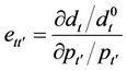
Demand management is most important technique to maximize benefit of both client and utility. To augment the utility revenue, maximum customer involvement is crucial. This simple and widely used model is based on an assumption in which demand will change linearly in respect to the elasticity. To formulate maximum customer involvement, demand of customer is to be analyze against change in prices for must run and optional loads. The price elasticity of demand is defined as the proportion of change in demand to the change in price.

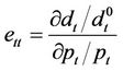
Logarithmic modeling of elastic load:
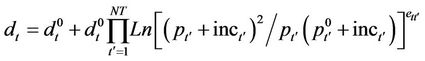
If customer demand changes from  to
to  based on incentive
  offered by utility so;
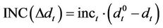
The prize incentive attracts the consumer so total incentive  function is given as;
Customer benefit for participating in DR program will be;
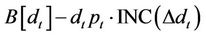
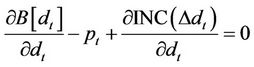
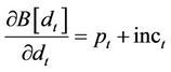
Combining the optimum customer behavior that leads to yields
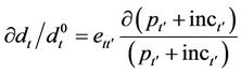
Parameter η is DR potential which can be entered to model as follows:
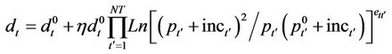
Larger the value of η means the more customer tendency to reduce or shift consumption from one hour to the other.
4.2. For Fixed Loads
For non shift able or must run loads we have elasticity known as “self elasticity” as [10] describes it.
As in our FEDRP must run loads price remain fixed and invariant of peak and off-peak hours so demand at any time for must run(base) loads will be given as
 (11)
(11)
So, demand for base loads will remain same through peak and off-peak hours and eventually customer’s participation increases in FEDRP.
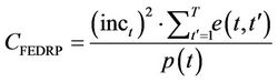
4.3. Cost of Customer Participation
 (12)
(12)
4.4. Demand Modeling of RAN
In a residential setup demand of electricity vary with consumer level, for a same price at some definite interval demand of a home may be different from other home. In our proposed FEDRP demand (Dh) of consumer is alienated into two portions, must run loads demand (df) and optional load demand (dv);
 (13)
(13)
In Figure 1(a) price of electricity is changing with the demand for variable loads with change in price in such a way that . d1 is demand of customer during peak hours where price increases which ultimately result in less customer’s demand and for d2, d3 and d4 end user’s demand is increased due to decreased prices, and for fixed loads as described in Figure 1(b) price remain same during peak and off peak hours.
In Figure 2 residential area setup is modeled such that demand of consumers is varying such that:
 (14)
(14)
 (15)
(15)
at different intervals will be:
 (16)
(16)
where “i” determine the period of time that customer demand during interval d1, d2, d3, and d4.
Now for second home demand considering both optional and must run load will be:
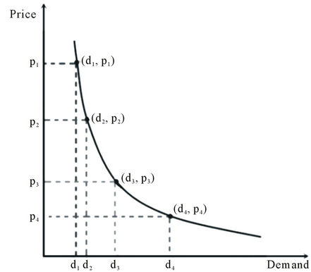 (a)
(a)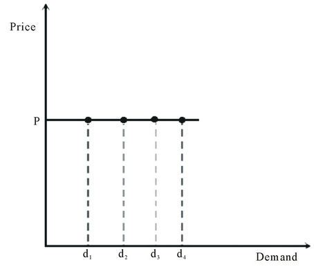 (b)
(b)
Figure 1. (a) Demand and price curve for optional (variable) loads; (b) Demand and price curve for fixed (must run) loads.
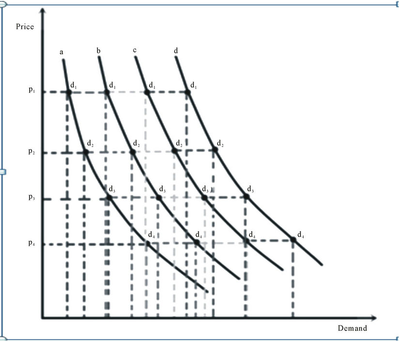
Figure 2. Demand and price curve for variable loads four homes in RAN.
 (17)
(17)
Similarly demands of home three and four are given as:
 (18)
(18)
 (19)
(19)
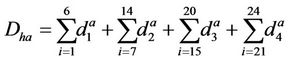
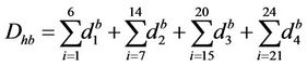
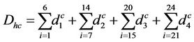
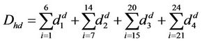
so the total fixed demand and variable demand for RAN during 24 hours is given as;
 (20)
(20)
Above equation describes the fixed demand in RAN during 24 hours similarly variable demand during a day is expressed as;
 (21)
(21)
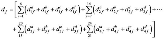
So total demand of these homes in residential setup from (16)-(19) will be:
 (22)
(22)
As total demand is equal to total fixed and total variable demand
 (23)
(23)
By simplifying above equation.
So total demand of these homes in residential setup from (16)-(19) will be:
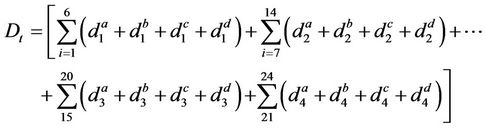 (24)
(24)
Considering total demand for residential setup of “m” homes with different demands during “4” intervals in 24 hours is described as
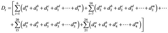 (25)
(25)
Equation (22) shows the total demand of “m” homes during 24 hours at four different intervals.
4.5. Utility Revenue
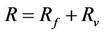
Scope of this article is to increase utility revenue along with the maximum customer satisfaction. In FEDRP utility revenue is of two types, first that utility obtain from fixed or “must run” loads and other revenue from variable or “optional” loads. This means that revenue and benefit of utility will be given as:
In proposed model company revenue is of two types, first that utility obtain from fixed or “must run” loads and other revenue from variable or “optional” loads. This means that revenue will be given as:
 (26)
(26)
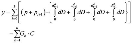
Taking into consideration the demands of four homes and their respective revenues at four intervals is calculated as:
Revenue from fixed (must run) loads will be:
 (27)
(27)
Revenue from variable (optional) loads will be:
 (28)
(28)
Using ,
,  in (23):
 (29)
(29)
For “m” homes revenue to utility at four intervals is described as
 (30)
(30)
Benefit function for utility is given as:
Profit = Revenue – Total operating cost
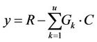 (31)
(31)
 (32)
(32)
5. Numerical Results and Simulation
In this section numerical and graphically study has been evaluated considering FEDRP. For this purpose daily load curve of Pakistani local grid has been taken for this simulation studies. The curve is divided into three sections as low load, off load and peak load periods as shown in Table 1 and energy prices are taken in rupees in different periods.
The selected values of self and cross elasticity’s have been shown in Table 2.
Fairness index has been calculated for fair emergency demand response program as follows:
Fairness index (FI) in [4] is described as ratio of customers whose demand is satisfied to total number of customers. Utility should effectively manage the customers demand weather for must run or optional loads. Fairness index given as
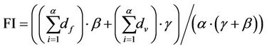 (33)
(33)
where β, γ are the priority of different loads and α is number of total customers. Considering the case for example in peak hours fixed load demand of 40 customers are satisfied and optional needs for 30 customers satisfied, and also priority of fixed load is twice of optional load [6], then FI = 0.91. The client contentment for no mandatory load depends on price variation for this load during peak and off-peak hours. Higher the prices less will be the demand of customer, for satisfying its optional load.
Total numerical analysis of daily load curve has been evaluated in Table 3 which shows utility fixed and variable revenues (Rf and Rv) under different cases of incentives given to clients for program participation. Initial fixed and variable demands (Dfi and Dvi) for the utility is shown with zero dollar incentives but the important thing is that as giving 25 dollar incentive for peak reduction to clients, Dv shifts tremendously as compared to 10 and 20 dollar incentives.
Total energy and peak reductions have been calculated in Table 4.
Figures 3-5 show the total variable demand analysis when different cases of consumer participation have been taken under different scenarios of incentives given by
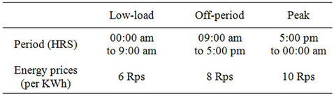
Table 1. Energy prices of daily load curve.
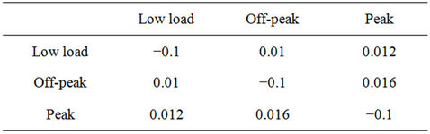
Table 2. Self and cross elasticity’s.
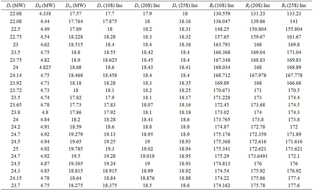
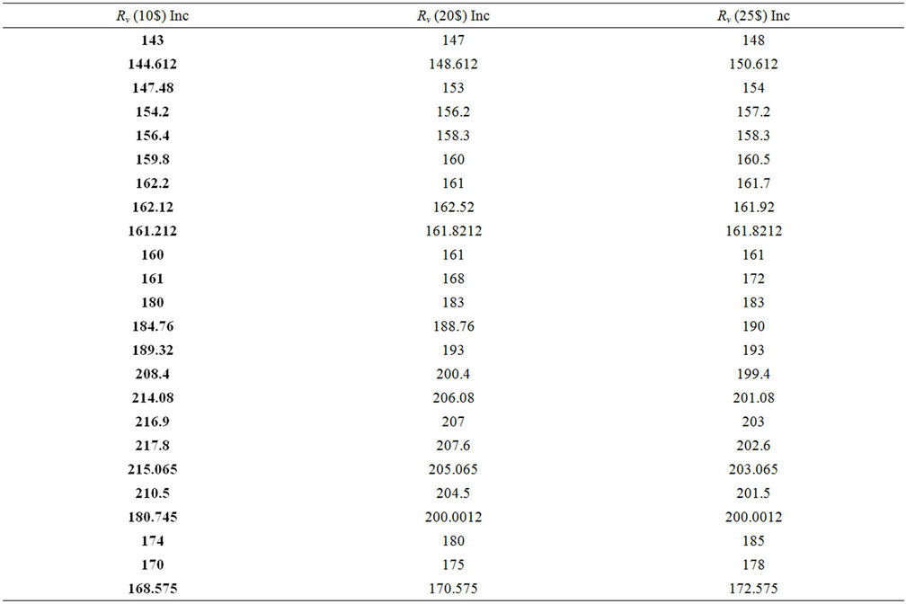
Table 3. Total numerical analysis of load curve.
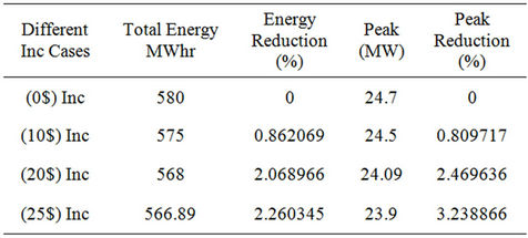
Table 4. Energy and peak reductions in % with different scenarios.
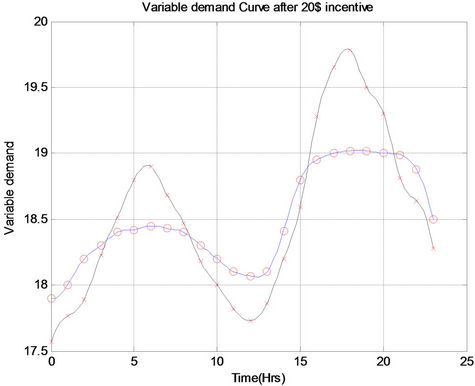
Figure 3. Variable demand for 20$ incentive.
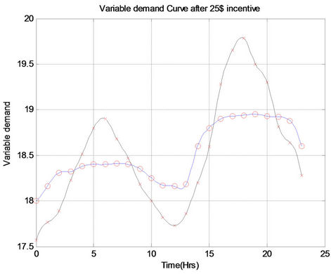
Figure 4. Variable demand for 25$ incentive.
the utility company to those customers who sign up the contract for FEDRP. Incentives in the form of 10, 20 and 25 dollars are given to the participants to reduce their variable load during emergency or peak hour. It has been analyzed in these figures that energy of daily load during peak hours has been sufficiently reduced and is shifted to off peak periods. Giving more incentives has permitted consumers to shift their load to off peak period. Similarly, Figures 6-8 show fixed revenues generated for utility company offering the program under different cases of incentives. The cases of variable revenues generated to utility from customer’s participation using their variable load has been calculated numerically and analyzed graphically as demonstrated in Figures 9 and 10. In all the analysis cases of incentives are compared clearly with non incentive cases which proves the whole scenario.
6. Conclusion
In this paper utility revenue and profit is modeled considering RAN for different user levels consumption, also demand of consumer is modeled mathematically and graphically. As consumer participation and satisfaction in DR program is basic tool to measure competitiveness for
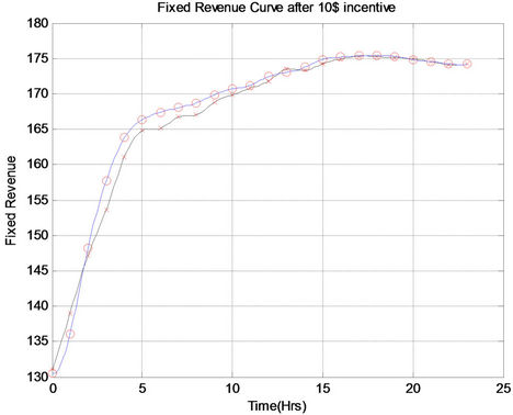
Figure 5. Fixed revenue for 10$ incentive.
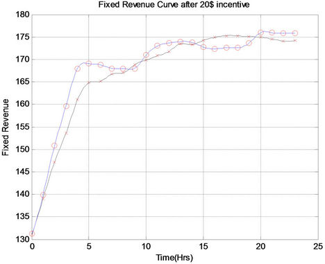
Figure 6. Fixed revenue for 20$ incentive.
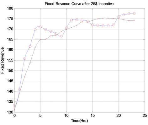
Figure 7. Fixed revenue for 25$ incentive.
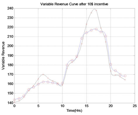
Figure 8. Variable revenue for 10$ incentive.
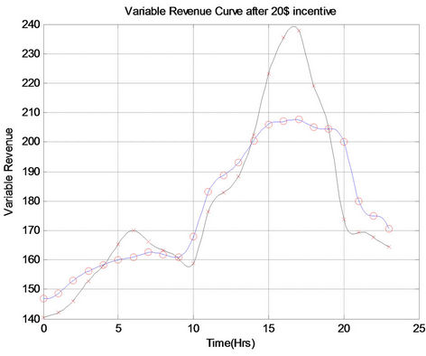
Figure 9. Variable revenue for 20$ incentive.
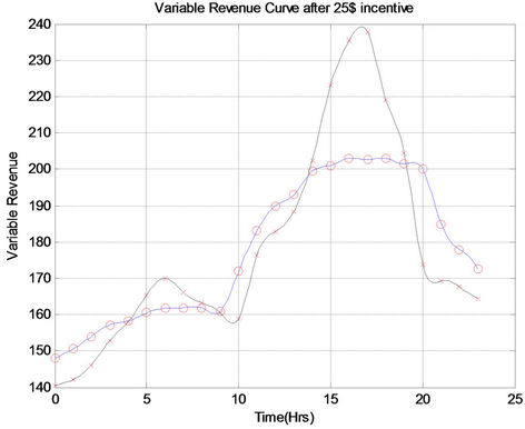
Figure 10. Variable revenue for 25$ incentive.
any DR program in market, so in this article end user participation is represented graphically with the comparison of initial demand before FEDRP. For customer contentment fairness index of the FEDRP is also calculated. Demand curve of FEDRP is plotted and also modeled numerically and compared with the existing EDRP.
7. Acknowledgements
The special thank goes to Dr. Imdad and Engr. Osama Bin Naveed who supported us in providing help in the preparation regarding to this article. We are also thankful to Mr. Istiaq Khan and Mr. Abdul Rehman as they have made a great contribution throughout our work especially in editing the text and paper formatting.
REFERENCES
- J. Pelletier, “ZigBee Powered Smart Grids Coming to a Home near You,” 2009.
- Zubair Md. Fadlullah, Mostafa M. Fouda, Nei Kato, Akira Takeuchi, Noboru Iwasaki, and Yousuke Nozaki, “Toward Intelligent Machine-to-Machine Communications in Smart Grid,” IEEE Communications Magazine, 2011.
- M. H. Albadi and E. F. El-Saadany, “A Summary of Demand Response in Electricity Markets,” Electric Power Systems Research, Vol. 78, No. 11, 2008, pp. 1989-1996. doi:10.1016/j.epsr.2008.04.002
- US Department of Energy, “Benefits of Demand Response in Electricity Markets and Recommendations for Achieving Them: A Report to the United States Congress Pursuant to Section 1252 of the Energy Policy Act of 2005,” 2006.
- J. J. Conti, P. D. Holtberg, J. A. Beamon, A. M. Schaal, G. E. Sweetnam and A. S. Kydes, “Annual Energy Outlook with Projections to 2035, Report of US Energy Information Administration (EIA),” 2010. http://www.eia.doe.gov
- Charles River Associate, “Primes on Demand Side Management with an Emphasis on Price Responsive Programs,” Report Prepared for the World Bank, Washington DC, CRA No. 006090. http://www.worldbank.org
- G. Thomas and P. E. Bellarmine, “Load Management Techniques,” Proceedings of the IEEE Southeastcon, Nashville, 7-9 April 2000, pp. 139-145.
- G. T. Bellarmine and N. S. S. Arokiaswamy, “Load Management,” Wiley Encyclopedia of Electrical and Electronics Engineering, Vol. 11, 1999, pp. 482-494.
- M. A. A. Pedrasa, T. D. Spooner and I. F. MacGill, “Coordinated Scheduling of Residential Distributed Energy Resources to Optimize Smart Home Energy Services,” IEEE Transactions on Smart Grid, Vol. 1, No. 2, 2010, pp. 134-143. doi:10.1109/TSG.2010.2053053
- A.-H. Mohsenian-Rad, V. W. S. Wong, J. Jatskevich and R. Schober, “Optimal and Autonomous Incentive-Based Energy Consumption Scheduling Algorithm for Smart Grid,” Innovative Smart Grid Technology, Gaithersburg, 19-21 January 2010, pp. 1-6.
- M. Erol-Kantarci and H. T. Mouftah, “Wireless Sensor Networks for Cost-Efficient Residential Energy Management in the Smart Grid,” IEEE Transactions on Smart Grid, Vol. 2, No. 2, 2011, pp. 314-325.
- A.-H. Mohsenian-Rad and A. Leon-Garcia, “Optimal Residential Load Control with Price Prediction in RealTime Electricity Pricing Environments,” IEEE Transactions on Smart Grid, Vol. 1, No. 2, 2010, pp. 120-133. doi:10.1109/TSG.2010.2055903
- A. Molderink, V. Bakker, M. G. C. Bosman, J. L. Hurink, and G. J. M. Smit, “Management and Control of Domestic Smart Grid Technology,” IEEE Transactions on Smart Grid, Vol. 1, No. 2, 2010, pp. 109-119. doi:10.1109/TSG.2010.2055904
- S. Tompros, N. Mouratidis, M. Draaijer, A. Foglar and H. Hrasnica, “Enabling Applicability of Energy Saving Applications on the Appliances of the Home Environment,” IEEE Network, Vol. 23, No. 6, 2009, pp. 8-16. doi:10.1109/MNET.2009.5350347
- E. Shayesteh, A. Yousefi, M. P. Moghaddam and M. K. Sheikh-El-Eslami, “ATC Enhancement Using Emergency Demand Response Program,” IEEE Power Systems Conference and Exposition, Seattle, 15-18 March 2009, pp. 1-7.
- M. H. Albadi and E. F. El-Saadany, “Demand Response in Electricity Markets: An Overview,” IEEE Power Engineering Society General Meeting, Tampa, 24-28 June 2007, pp. 1-5.
- US Dept of Energy, “Benefits of Demand Response in Electricity Markets and Recommendation for Achieving Them. A Report to the US Congress,” 2006.
- R. Tyagi and J. W. Black, “Emergency Demand Response for Distribution System Contingencies,” IEEE PES Transmission and Distribution Conference and Exposition, New Orleans, 19-22 April 2010, pp. 1-4.
- S. Valero, M. Ortiz, et al., “Methods for Customer and Demand Response Policies Selection in New Electricity Markets,” Generation, Transmission & Distribution, Vol. 1, No. 1, 2007, pp. 104-110.
- P. Moses and M. S. Moasum, “Load Management in Smart Grids Considering Harmonic Distortion and Transformer Detering,” IEEE Innovative Smart Grid Technologies, Gaithersburg, 19-21 January 2010, pp. 1-7.
Nomenclature
 : Initial demand;
 : Initial price;
 : Price change in period t;
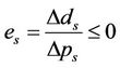
 : Demand change in period s;
 : Elasticity;
 : Change in demand in i-th hour after FEDRP;
 : Demand in i-th hour before FEDRP (KWh);
 : Demand in i-th hour after FEDRP (KWh);
 : Incentive in i-th hour ($/Kwh);
 : Penalty in i-th hour ($/Kwh);
 : Contract level;
 : Client income in i-th hour;
 : Price before FEDRP in i-th hour ($/Kwh);
 : Price after FEDRP in i-th hour ($/Kwh);
 : Self elasticity in i-th hour;
 : Demand cross elasticity between i-th and j-th hour;
 : Demand for must run load;
 : Demand for variable load;
 : Total demand of residential setup (MWH);
 : Total revenue to Utility ($);
 : Supply generation of unit k;
 : Generation cost;
 : Profit to Utility ($).