Journal of Signal and Information Processing
Vol. 4 No. 2 (2013) , Article ID: 30999 , 9 pages DOI:10.4236/jsip.2013.42022
Chirplet Signal and Empirical Mode Decompositions of Ultrasonic Signals for Echo Detection and Estimation
![]()
1Department of Electrical and Computer Engineering, Bradley University, Peoria, USA; 2Department of Electrical and Computer Engineering, Illinois Institute of Technology, Chicago, USA.
Email: ylu2@bradley.edu, erdal@ece.iit.edu, sansonic@ece.iit.edu
Copyright © 2013 Yufeng Lu et al. This is an open access article distributed under the Creative Commons Attribution License, which permits unrestricted use, distribution, and reproduction in any medium, provided the original work is properly cited.
Received December 31st, 2012; revised February 1st, 2013; accepted February 10th, 2013
Keywords: Ultrasound; Hilbert Time-Frequency Representation; Empirical Mode Decomposition; Chirplet Signal Decomposition; Detection; Estimation
ABSTRACT
In this study, the performance of chirplet signal decomposition (CSD) and empirical mode decomposition (EMD) coupled with Hilbert spectrum have been evaluated and compared for ultrasonic imaging applications. Numerical and experimental results indicate that both the EMD and CSD are able to decompose sparsely distributed chirplets from noise. In case of signals consisting of multiple interfering chirplets, the CSD algorithm, based on successive search for estimating optimal chirplet parameters, outperforms the EMD algorithm which estimates a series of intrinsic mode functions (IMFs). In particular, we have utilized the EMD as a signal conditioning method for Hilbert time-frequency representation in order to estimate the arrival time and center frequency of chirplets in order to quantify the ultrasonic signals. Experimental results clearly exhibit that the combined EMD and CSD is an effective processing tools to analyze ultrasonic signals for target detection and pattern recognition.
1. Introduction
Different time-frequency analysis methods such as shorttime Fourier transform (STFT), Wigner-Ville distribution (WVD), and wavelet transform (WT) have been utilized to examine nonstationary signals often encountered in ultrasonic imaging applications [1-4]. For example, Berriman et al., investigated ultrasonic non-destructive testing of concrete using STFT and WVD [1]. Similarly, Kuang et al., used STFT and wavelet packet filters for frequency measurement in a Doppler tracking system [2]. Furthermore, time-frequency analysis has been shown to extract critical frequency-diverse information which can be used to discriminate clutter and target echoes in ultrasonic detection applications [3]. However, it remains a very significant problem to obtain a general transform basis which is adaptive to nonstationary and interfering narrowband, broadband and dispersive echoes corrupted by noise. Lately, as an alternative to classical time-frequency distributions, an empirical mode decomposition (EMD) technique [4] has been used for signal analysis. EMD splits the signal into a series of intrinsic mode functions (IMF) by using local signal attributes such as the location of the extreme points and zero crossings. Estimated IMFs are oscillatory and adaptive to the characteristics of the signal. Hence, the time-frequency distribution of the signal can be obtained from the Hilbert spectrum of estimated IMFs [5,6].
The EMD has been explored in the applications of medical imaging and diagnostics [7,8], time-frequency analysis of encountered waves [9], underwater acoustic feature extraction [10], image watermarking [11], power systems [12], vibration analysis for structural health monitoring [13], audio source separation [14] and ultrasonic nondestructive evaluation [15]. Although the algorithm is successfully utilized in diverse application areas, it lacks a well-established theoretical analysis [16-18]. Therefore, any new application of EMD requires rigorous verification and evaluation of the method. In this paper, the EMD algorithm is introduced to characterize ultrasonic backscattered echoes which are often intrinsically oscillatory and nonstationary. Furthermore, the performance of EMD has been compared to the estimation results obtained from chirplet signal decomposition algorithm [19-22]. Chirplet is a type of signal frequently encountered in ultrasonic applications. The six parameters of a chirplet [19], i.e., time-of-arrival, center frequency, amplitude, bandwidth factor, chirp rate and phase, can be used to represent a broad range of ultrasonic echo shapes including narrowband, broadband and dispersive echoes. In this study, the estimated echo parameters are used to substantiate the sensitivity of EMD to different type of echoes in presence of noise.
2. Empirical Mode Decomposition of Ultrasonic Chirp Echoes
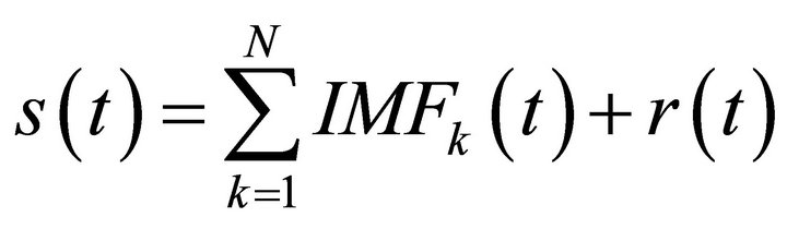
The objective of the EMD is to decompose a highly convoluted, multi-component ultrasonic signal, ![]() , into N series of IMFs.
, into N series of IMFs.
 (1)
(1)
Here ![]() denotes the residue of signal reconstruction; and
denotes the residue of signal reconstruction; and  denotes the kth IMF function. The process to obtain these IMFs is an iterative decomposition process [5]. Figure 1 shows the flowchart of EMD process (known as sifting process) to estimate IMFs. The steps involved in the sifting process of signal
 ![]() are:
are:
1) Prepare signal  for sifting process, where x(t) = s(t), set the iteration index j = 1;
2) Find all the local maxima and local minima of ;
;
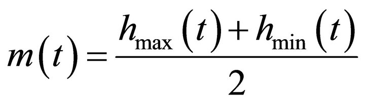
3) Interpolate the local maxima to form the maxima envelop, . Similarly, the minima envelop,
  , is obtained. Hence, the mean sequence,
  , can be obtained from
  and
and ;
;
4) 
5) Subtract the mean envelop,  , from the signal,
  such that
 . Check if
  is an IMF (see below for IMF conditions); If
  is an IMF, go to Step 5; otherwise, go to Step 2 and update
 , repeat Steps 2-4.
6) Save the IMF result: , update the iteration index
 , subtract the estimated IMFs from signal
 ![]() to obtain residue
to obtain residue
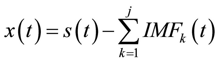 (2)
(2)
7) Check the residue  from Step 5. If
  is a constant or monotonic function, save all IMFs and complete the sifting process; otherwise, go to Step 2.
Steps 1 through 6 allow the sifting process to isolate time-varying signal features and obtain the intrinsic oscillation.
IMF Conditions:
To be an IMF, the signal must satisfy the following conditions:
1) 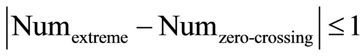
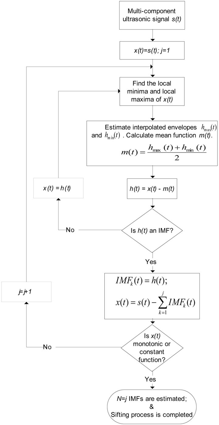
Figure 1. Flowchart of empirical mode decomposition estimation process.
where  is the number of local extreme points (includes local maxima and local minima), and
  is the number of cross-zero points.
2) 
where  is the envelope interpolated by all local maxima,
  is the envelope interpolated by all local minima,
  is the mean sequence of local maxima and minima envelops, and
 ![]() is a sufficiently small positive value close to zero.
is a sufficiently small positive value close to zero.
In practice, the signal segment and noise may override the realization of condition 1) and it is also problematic to get an absolute-zero mean sequence  for the condition 2) of IMF. Therefore, different methods have been used as an alternate to conditions 1) and 2) and to stop the estimation searching process of IMF [6]. One method is to check if the mean square error of
  between two successive iterations is smaller than a predefined value. A practical alternative method is to check if
  satisfies the condition 1) of IMF for a predefined number of successive iterations. In this study, a predefined number of iterations are used to compensate for the condition 2) of IMF.
To introduce the EMD process into ultrasonic pulseecho system, it is useful to analyze the EMD effect on ultrasonic chirp echoes, a type of signal often encountered in ultrasonic backscattered signal accounting for narrow-band, broad-band, and dispersive echoes.
An ultrasonic chirp echo can be modeled as:
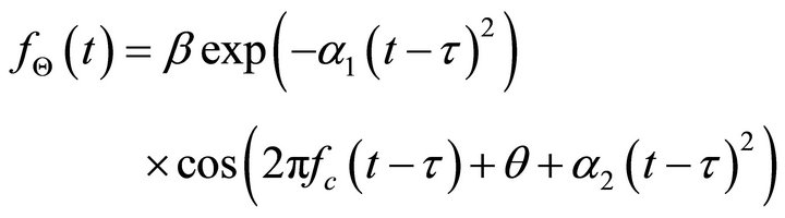 (3)
(3)
where 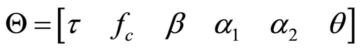 denotes the parameter vector,
 ![]() is the time-of-arrival,
is the time-of-arrival,  is the center frequency,
  is the amplitude,
  is the bandwidth factor,
  is the chirp-rate, and
  is the phase.
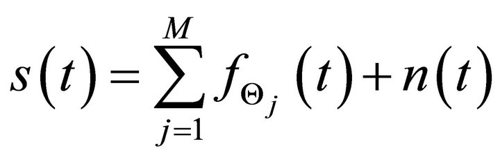
Similarly, a signal consisting of multiple chirp echoes can be simulated and decomposed using EMD. The simulated signal, ![]() , can be written as follows
, can be written as follows
 (4)
(4)
where  denotes the jth chirp echo,
  denotes a noise.
In fact, the Gaussian-envelop chirplet echo,  , satisfies IMF conditions 1 and 2. The ultrasonic chirplet echo can be viewed, for all practical purposes, as a band-limited and time-limited function. Signals consisting of multiple partially overlapped chirplets require multiple IMFs and the number of IMFs not only depends on the number of the echoes, but also depends on the degree of overlap between echoes. Figure 2 shows the IMF results of two overlapped chirplets with the following parameters:

and

The first IMF reveals the non-overlapping portion of both chirplets and it takes one additional IMF with low frequency components to compensate for the asymmetric portion representing the overlapped. It is a non-parametric process to generate IMFs. One may conclude IMFs tracks the oscillation within the signal, but it cannot characterize the degree of overlap among multiple echoes. Consequently, it cannot be used with certainty to estimate chirplet parameters. The EMD tracks the irregularity in signal instead of decomposing it into individual chirplets. The Fourier spectrum of these IMFs (see Figure 2) shows that IMFs track different frequency bands associated with time-of-arrival of echoes.
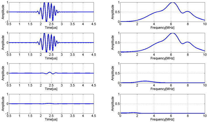
Figure 2. EMD result of two overlapping chirplet echoes (left column: from top to bottom: simulated signal, IMF #1, IMF #2, and residue; right column: Fourier spectrum of the corresponding signals in left column).
The EMD is similar to a filter-bank process sweeping from higher frequency bands to lower frequency bands. This can be advantageous for denoising the signal. Figure 3 demonstrates that the performance of the EMD when applied to chirplet echoes with the following parameters:

and

plus a white Gaussian noise with SNR of 10dB. To further the evaluation of EMD results for ultrasonic signals, Hilbert spectrum, discussed in next section, is used to perform the time-frequency analysis.
3. Hilbert Time-Frequency Representation of Chirp Echoes
Hilbert time-frequency representation [23] provides critical information about chirplet echoes such as the center frequency and time-of-arrival parameters. Therefore, Hilbert transform can be successfully used in ultrasonic echo detection and estimation applications. In this section, we first discuss chirplet echo parameter sensitivity and then demonstrate that Hilbert transform can be used in conjunction with EMD for ultrasonic signal analysis.
To explore the behavior of the chirplet parameters, a simulation has been conducted to examine the change of reconstruction error as each parameter is altered for a single ultrasonic chirp echo [22]. In the case of the parameter deviation varying from −10% to 10% of the actual value, Figure 4 shows how the reconstruction error evolves with the alteration of each single parameter. It can be seen that the time-of-arrival dominates the effects on reconstruction error, compared with other parameters. Hence, the time-of-arrival, ![]() , is the most critical parameter to be estimated, followed by the center frequency
, is the most critical parameter to be estimated, followed by the center frequency , the amplitude
 , the chirp rate
 , the phase
 , and the bandwidth factor
 .
.
To analyze the time-frequency property of signal,  , Hilbert transform is applied to the signal, and the analytic signal,
  , can be defined as
 (5)
(5)
where  denotes the Hilbert transform. Therefore, the chirplet analytic signal,
  can be approximated with reasonable accuracy (when center frequency is larger the chirplet bandwidth [23,25-27]) as
 (6)
(6)
where
 (7)
(7)
 (8)
(8)
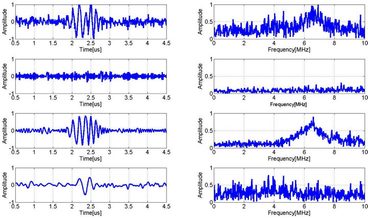
Figure 3. EMD results of a noisy signal with two overlapping chirplet echoes (left column: from top to bottom: simulated signal, IMF #1, IMF #2, and residue; right column: Fourier spectrum of the corresponding signal in left column).
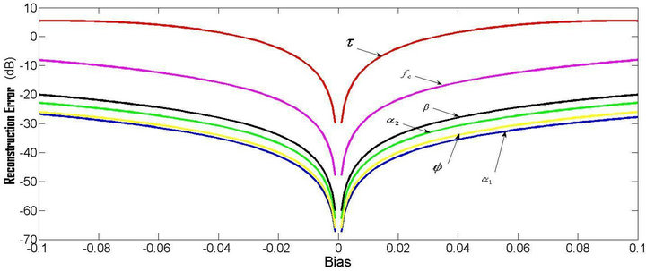
Figure 4. Parameter behavior analysis for a single noisy chirp echo.
Let  denotes the Hilbert time-frequency representation of the signal,
  , which is
![]() (9)
(9)
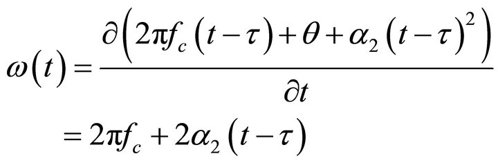
The maximum of  can be obtained by taking derivatives of the
  with respect to
 .
.
 (10)
(10)
The solution of Equation (10) leads to an estimation of time-of-arrival,
 (11)
(11)
and using Equation (8), the frequency at the time arrival represent the center frequency
 (12)
(12)
Equations (11) and (12) indicates that Hilbert timefrequency (TF) representation can be used to analyze ultrasonic chirp signal and reveal the two most critical parameters, i.e., time-of-arrival and center frequency.
Similarly, in a multi-component ultrasonic signal, ![]() , which includes a linear expansion of chirp echoes, Hilbert TF representation can be obtained from its analytical signal
, which includes a linear expansion of chirp echoes, Hilbert TF representation can be obtained from its analytical signal .
.
 (13)
(13)
where , which includes
  chirp echoes;
  denotes the amplitude of jth chirp echo; and
  denotes the frequency of jth chirp echo.
To demonstrate the performance of the Hilbert TF representation in ultrasonic signal analysis, ultrasonic chirp echo is simulated in Figure 5, where positive or negative chirp rate models the dispersive effect in ultrasonic testing of materials. This figure shows the estimated time-of-arrivals and center frequencies closely match the actual values used in simulating these signals.
4. Ultrasonic Experimental Results
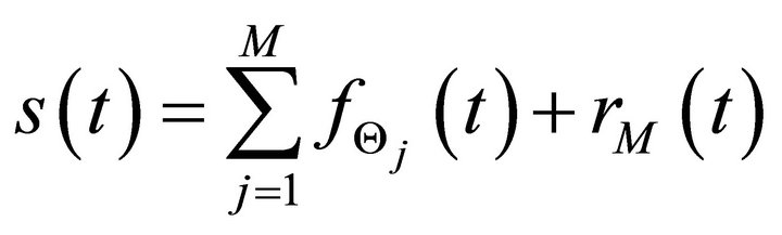
To evaluate the performance of EMD in analysis of ultrasonic backscattered signals, chirplet signal decomposition (CSD) is included for the comparison purposes in this study. The CSD algorithm [18] is utilized to decompose the ultrasonic signal, ![]() , into a linear expansion of chirp echoes and efficiently estimate the parameter vectors of these echoes.
, into a linear expansion of chirp echoes and efficiently estimate the parameter vectors of these echoes.
 (14)
(14)
where  denotes the residue of the signal reconstruction after estimating M successive ultrasonic chirp echoes,
 .
.
An experiment is conducted to acquire ultrasonic backscattered signal from a steel block with a flat-bottom hole (i.e., target) using a 5 MHz transducer and sampling rate of 100 MHz. Figure 6 shows the experimental data superimposed with the reconstructed signal using CSD algorithm consisting of 6 chirplets, compared with the experimental data superimposed with the reconstructed signal using EMD consisting of 3 IMFs. It can be seen that both methods can successfully perform signal decomposition on the experimental data. Moreover, the parameters of the target echo are shown in the first row of Table 1, which lists the estimated parameters of chirplets using CSD algorithm. The target echo exhibits a lower center frequency (Echo #1 in the table, time arrival = 2.7618 ms, center frequency = 4.3513 MHz) due to the effect of frequency-dependent attenuation compared to the surrounding scattering echoes that often exhibit higher center frequencies [28].
The EMD has been applied to the same experimental data set. The results from EMD are shown in Figure 7,
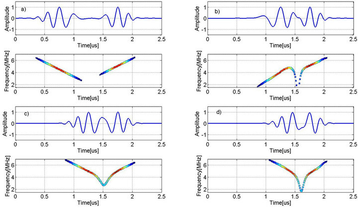
Figure 5. Hilbert TF representation of ultrasonic chirp (Row 2: Hilbert TF representation of the ultrasonic chirp echoes in Row 1; Row 4: Hilbert TF representation of the ultrasonic chirp echoes in Row 3).
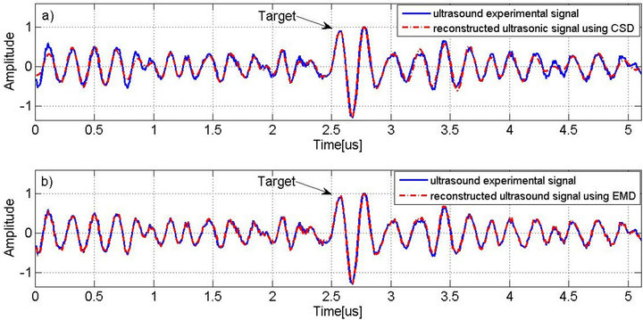
Figure 6. a) Ultrasonic experimental data superimposed with the reconstructed signal using CSD algorithm; b) Ultrasonic experimental data superimposed with the reconstructed signal using EMD.
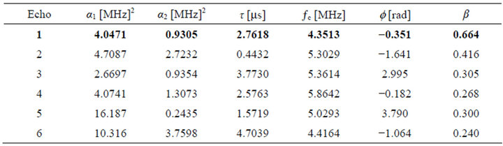
Table 1. Estimated parameters of chirplets (CSD method).
where the ultrasonic experimental data, IMF #1, IMF #2, IMF #3 and residue function are plotted from top to bottom. It can be seen that the dominant echo location in IMF #1 is around 2.76 microseconds, which is close to the time of arrival, ![]() , of the target echo (see parameters of Echo #1 in Table 1). Furthermore, the Hilbert timefrequency representation of the ultrasonic signal (see Figure 8b) shows that the target is emphasized in the
, of the target echo (see parameters of Echo #1 in Table 1). Furthermore, the Hilbert timefrequency representation of the ultrasonic signal (see Figure 8b) shows that the target is emphasized in the
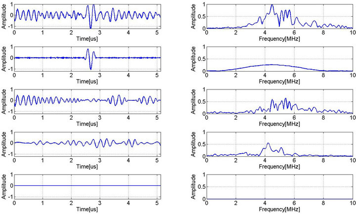
Figure 7. EMD results of ultrasonic backscattered signal (left column: from top to down: experimental data, IMF #1, IMF #2, IMF #3, and residue; right column: Fourier spectrum of the corresponding signal in left column).
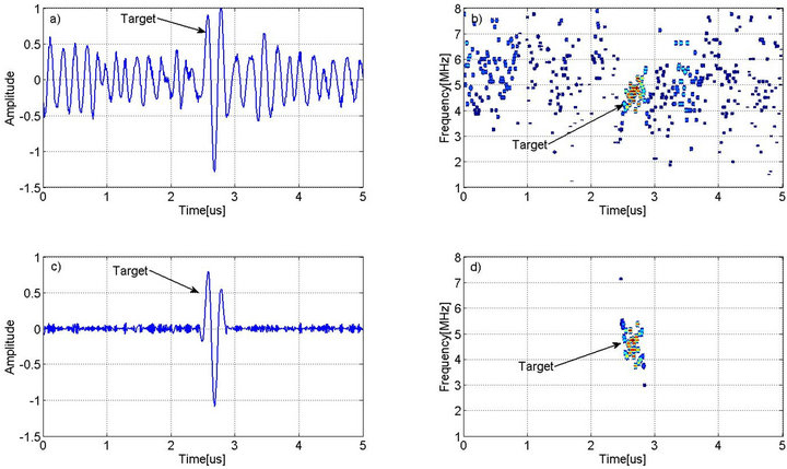
Figure 8. a) Ultrasonic backscattered signal; b) Hilbert time-frequency representation of ultrasonic backscattered signal in a); c) IMF #1 from EMD results of ultrasonic backscattered signal in a); d) Hilbert time-frequency representation of IMF #1 in c).
Hilbert time-frequency domain. It also can be seen that the information of the target time-frequency characteristic is smeared by the surrounding scattered echoes caused by the microstructure of the test object. After the EMD process, by further examining the Hilbert time-frequency representation of the IMF #1, the useful information of the target, such as center frequency and time-of-arrival, is clearly displayed in Figure 8d.
The center frequency of the target is around 4.4 MHz and the time-of-arrival of the target is around 2.76 microseconds, which is in agreement with the estimated parameters using CSD algorithm. Therefore, combining with Hilbert time-frequency analysis, the EMD can successfully analyze ultrasonic backscattered signal and obtain useful information related to the target. However, unlike CSD algorithm, the EMD and Hilbert time-frequency representation cannot decompose the ultrasonic backscattered signal into a well-defined chirplet model and cannot estimate the specific chirplet parameters. These parameters are critical for nondestructive testing and quantitative material characterization.
5. Conclusion
In this study, the EMD has been introduced to analyze ultrasonic backscattered signals for ultrasonic nondestructive evaluation of materials. Numerical and analytical results indicate that the EMD is a unique tool for ultrasonic signal analysis and is sensitive to center frequency of echo, and their interference amongst them. Compared with CSD algorithm, the EMD has limitation on signal decomposition and accurate parameter estimation. The EMD is a unique and effective method to track signal changes while the estimation results obtained by CSD algorithm quantify the ultrasonic signals accounting for narrow-band, broad-band, and dispersive echoes.
REFERENCES
- J. Berriman, D. Hutchins, N. Adrian, G. Tat and P. Purnell, “The Application of Time-Frequency Analysis to the Air-Coupled Ultrasonic Testing of Concrete,” IEEE Transactions on Ultrasonics, Ferroelectrics, and Frequency Control, Vol. 53, No. 4, 2006, pp. 768-776.
- W. Kuang and A. Morris, “Using Short-Time Fourier Transform and Wavelet Packet Filter Banks for Improved Frequency Measurement in a Doppler Robot Tracking System,” IEEE Transactions on Instrumentation and Measurement, Vol. 51, No. 3, 2002, pp. 440-444. doi:10.1109/TIM.2002.1017713
- J. Saniie, D. T. Nagle and K. D. Donohue, “Analysis of Order Statistic Filters Applied to Ultrasonic Target Detection Using Split Spectrum Processing,” IEEE Transactions on Ultrasonics, Ferroelectrics, and Frequency Control, Vol. 38, No. 2, 1991, pp. 133-140. doi:10.1109/58.68470
- N. Huang, Z. Shen, S. Long, M. Wu, H. Shih, Q. Zheng, N. Yen, C. Tung and H. Liu, “The Empirical Mode Decomposition and the Hilbert Spectrum for Nonlinear and Non-Stationary Time Series Analysis,” Proceedings of Royal Society London, Vol. 454, No. 1971, 1998, pp. 903-995. doi:10.1098/rspa.1998.0193
- N. Huang and S. Shen, “Hilbert-Huang Transform and Its Applications, Interdisciplinary Mathematical Sciences,” World Scientific Publishing Co., The Singapore City, 2005.
- N. Huang and N. Attoh-Okine, “The Hilbert-Huang Transform in Engineering,” CRC Press, Taylor and Francis Publishing Group, Boca Raton, 2005.
- Y. Zhang, Y. Gao, L. Wang, J. Chen and X. Shi, “The Removal of Wall Components in Doppler Ultrasound Signals by Using the Empirical Mode Decomposition Algorithm,” IEEE Transactions on Biomedical Engineering, Vol. 54, No. 9, 2007, pp. 1631-1642. doi:10.1109/TBME.2007.891936
- H. Liang, Q. Lin and J. Chen, “Application of the Empirical Mode Decomposition to the Analysis of Esophageal Manometric Data in Gastroesophageal Reflux Disease,” IEEE Transactions on Biomedical Engineering, Vol. 52, No. 10, 2005, pp. 1692-1701. doi:10.1109/TBME.2005.855719
- M. Li, X. Gu and P. Shan, “Time-Frequency Distribution of Encountered Waves Using Hilbert-Huang Transform,” International Journal of Mechanics, Vol. 1, No. 2, 2007, pp. 27-32.
- G. Ge, E. Sang, Z. Liu and B. Zhu, “Underwater Acoustic Feature Extraction Based on Bidimensional Empirical Mode Decomposition in Shadow Field,” IEEE Proceedings of Signal Design and its Applications in Communcations, Chengdu, 23-27 September 2007, pp. 365-367.
- N. Bi, Q. Sun, D. Huang, Z. Yang and J. Huang, “Robust Image Watermarking Based on Multiband Wavelets and Empirical Mode Decomposition,” IEEE Transaction on Image Processing, Vol. 16, No. 8, 2007, pp. 1956-1966. doi:10.1109/TIP.2007.901206
- N. Senroy, “Generator Coherency Using the HilbertHuang Transform,” IEEE Transactions on Power Systems, Vol. 23, No. 4, 2008, pp. 1701-1708. doi:10.1109/TPWRS.2008.2004736
- R. Yan and R. Gao, “Hilbert-Huang Transform-Based Vibration Signal Analysis for Machine Health Monitoring,” IEEE Transactions on Instrumentation and Measurement, Vol. 55, No. 6, 2006, pp. 2320-2329. doi:10.1109/TIM.2006.887042
- M. Molla and K. Hirose, “Single-Mixture Audio Source Separation by Subspace Decomposition of Hilbert Spectrum,” IEEE Transactions on Audio, Speech, and Language Processing, Vol. 15, No. 3, 2007, pp. 893-900. doi:10.1109/TASL.2006.885254
- Y. Lu, E. Oruklu and J. Saniie, “Application of HilbertHuang Transform for Ultrasonic Nondestructive Evaluation,” IEEE Proceedings of Ultrasonics Symposium, Beijing, 2-5 November 2008, pp. 1499-1502.
- Y. Kopsinis and S. McLaughlin, “Investigation and Performance Enhancement of the Empirical Mode Decomposition Method Based on a Heuristic Search Optimization Approach,” IEEE Transactions on Signal Processing, Vol. 56, No. 1, 2008, pp. 1-13. doi:10.1109/TSP.2007.901155
- E. Delechelle, J. Lemonie and O. Niang, “Empirical Mode Decomposition: An Analytical Approach for Sifting Process,” IEEE Signal Processing Letters, Vol. 12, No. 11, 2005, pp. 764-767. doi:10.1109/LSP.2005.856878
- G. Rilling and P. Flandrin, “One or Two Frequencies? The Empirical Mode Decomposition Answers,” IEEE Transactions on Signal Processing, Vol. 56, No. 1, 2008, pp. 85-95. doi:10.1109/TSP.2007.906771
- Y. Lu, R. Demirli, G. Cardoso and J. Saniie, “A Successive Parameter Estimation Algorithm for Chirplet Signal Decomposition,” IEEE Transaction on Ultrasonics, Ferroelectrics, and Frequency Control, Vol. 53, No. 11, 2006, pp. 2121-2131. doi:10.1109/TUFFC.2006.152
- Y. Lu, E. Oruklu and J. Saniie, “Fast Chirplet Transform with FPGA-Based Implementation,” IEEE Signal Processing Letters, Vol. 15, 2008, pp. 577-580. doi:10.1109/LSP.2008.2001816
- Y. Lu, R. Demirli, G. Cardoso and J. Saniie, “Chirplet Transform for Ultrasonic Signal Analysis and NDE Applications,” IEEE Proceedings of Ultrasonic Symposium, Rotterdam, 18-21 September 2005, pp. 18-21.
- Y. Lu, R. Demirli and J. Saniie, “A Comparative Study of Echo Estimation Techniques for Ultrasonic NDE Applications,” IEEE Proceedings of Ultrasonic Symposium, Vancouver, 2-6 October 2006, pp. 536-539.
- L. Cohen, “Time Frequency Analysis: Theory and Applications,” Prentice Hall, Upper Saddle River, 1994.
- Y. Lu, R. Demirli and J. Saniie, “Efficiency and Sensitivity Analysis of Chirplet Signal Decompsotion for Ultraosnic NDE Applications,” IEEE Proceedings of Ultrasonic Symposium, Vol. 1, 2007, pp. 1590-1593.
- E. Bedrosian, “A Product Theorem for Hilbert Transforms,” Proceedings of IEEE, Vol. 51, No. 5, 1963, pp. 868-869.
- E. Hermanowicz and M. Rojewski, “On Bedrosian Condition in Application to Chirp Sounds,” Proceedings of 15th European Signal Processing Conference, Poznań, 3-7 September 2007, pp. 1221-1225.
- E. Oruklu, Y. Lu and J. Saniie, “Hilbert Transform Pitfalls and Solutions for Ultrasonic NDE Applications,” IEEE Proceedings of Ultrasonic Symposium, Rome, 20- 23 September 2009, pp. 2004-2007.
- J. Saniie and D. T. Nagle, “Analysis of Order-Statistic CFAR Threshold Estimators for Improved Ultrasonic Flaw Detection,” IEEE Transactions on Ferroelectrics and Frequency Control, Vol. 39, No. 5, 1992, pp. 618- 630. doi:10.1109/58.156180