Agricultural Sciences
Vol.5 No.4(2014), Article ID:43991,12 pages DOI:10.4236/as.2014.54037
Monitoring Heat Waves and Their Impacts on Summer Crop Development in Southern Brazil*
Anibal Gusso1,2,3#, Jorge Ricardo Ducati2,4, Mauricio Roberto Veronez3,5, Victor Sommer6, Luiz Gonzaga da Silveira Junior3,7
1Environmental Engineering, Vale do Rio dos Sinos University (UNISINOS), São Leopoldo, Brazil
2Center for Remote Sensing and Meteorological Research, Federal University of Rio Grande do Sul (UFRGS), Porto Alegre, Brazil
3VizLab-Advanced Visualization Laboratory, Vale do Rio dos Sinos University (UNISINOS), São Leopoldo, Brazil
4Astronomy Department, Federal University of Rio Grande do Sul (UFRGS), Porto Alegre, Brazil
5Graduate Program in Geology, Vale do Rio dos Sinos University (UNISINOS), São Leopoldo, Brazil
6Crop Breeding Foundation (Fundação Pró-Sementes), Passo Fundo, Brazil
7Graduate Program in Applied Computing, Vale do Rio dos Sinos University (UNISINOS), São Leopoldo, Brazil
Email: #anibalg@unisinos.br
Copyright © 2014 by authors and Scientific Research Publishing Inc.
This work is licensed under the Creative Commons Attribution International License (CC BY).
http://creativecommons.org/licenses/by/4.0/


Received 4 January 2014; revised 25 February 2014; accepted 12 March 2014
ABSTRACT
Periods in the soybean summer cycle that are sensitive to the occurrence of high temperatures were studied. An analysis was performed on the variability of soybean yields associated with crop canopy temperatures during key development periods. A land surface temperature (LST) data series from MODIS (Moderate Resolution Imaging Spectroradiometer) on the Aqua satellite was processed between 2003 and 2012 that covered the entire state of Rio Grande do Sul, in Brazil. Enhanced vegetation index (EVI) data from MODIS on the Terra satellite were used to monitor the LST during different phenological stages. Spatially interpolated maps of soybean yield distributions were generated using data obtained from Instituto Brasileiro de Geografia e Estatística (IBGE) at state and municipality levels. The results indicate that canopy-LST occurrence in mid-February, during the grain filling, is most correlated to yield reduction (R2 = 0.82 and RMSD = 14.4%). At the state level, the average yield is 2003 kg∙ha−1 with a standard deviation of 308 kg∙ha−1. The overall average of the canopy-LST is 305.0 K (31.8˚C) with a standard deviation of 1.9 K. The slope of the downward linear relationship between canopy-LST and yield was −28.7%. These results indicate that monitoring heat wave events can provide important information for characterising agriculture vulnerability.
Keywords: Land Surface Temperature; Soybean; Remote Sensing; Canopy; Vegetation Index; MODIS Data

1. Introduction
Weather fluctuations and other associated extreme events can cause severe losses to agricultural production with potential worldwide economic impacts [1] [2] . In Brazil, increases in the frequency of extreme events, such as the occurrence of high temperatures and reduced rainfall, are prone to produce severe effects on agricultural yields [3] [4] , especially soybeans and maize [5] . As a result, distortions and uncertainties in agricultural policies may increase losses and establish barriers for agricultural financing [6] due to unpredictable government policies which are a more important cause of domestic price volatility than world market price fluctuations [1] .
Under a climate change scenario, the physical parameters of the earth’s surface, such as temperature, water availability and evapotranspiration, will change over the future decades [7] [8] . These changes can restrict crop development and reduce yields, which could be adversely affected as canopy temperature fluctuations often exceed the optimum range [9] . Thus, a better understanding of plant responses to the combined effect of drought and heat stress is pertinent [10] to the management of potential regional climate risks in the coming decades [3] [11] [12] .
The stress caused by high temperature occurrences has impacts on agricultural yields, even when the average temperature reaches one or two degrees above the ideal for the culture [13] -[15] . However, the quantitative assessment of production losses and impacts on yields from the duration and intensity of heat waves is still an issue [16] [17] .
Rio Grande do Sul State (RS hereafter) is the third largest producer of soybeans in Brazil and accounted for approximately 18% of the national production in 2012 [18] . Although the production was 11.62 million tons in 2011, it reached a yield average at the state level of 2845 kg∙ha−1. The historical average from 2003 to 2012 was only 2097 kg∙ha−1 [18] . During most years, the frequency and intensity of rainfall from sowing to harvest have been variable and often insufficient for the full development of culture [19] . For this purpose, improvements in the management capacity and strategies are essential to benefit from favourable weather conditions and mitigate impacts of non-favourable conditions [20] [21] .
In the Rio Grande do Sul State (RS), the large inter-annual variability of rainfall is mainly due to El Niño and La Niña occurrences, which cause yield fluctuations in southern Brazil [20] -[22] ; there, the most impacted crops are usually soybean and maize [20] in the summer. Prolonged drought effects on the summer crop in 2005 caused a decrease of approximately 75% in the soybean grain production [23] . Although weather fluctuations, such as high temperature occurrences and water stress, are not always problematic [16] , heat waves that may or may not be associated with droughts are increasingly gaining interest in scientific publications [24] due to the need for sustainable agriculture management and an assessment of the vulnerability to future international demands [4] .
The crop development profile of vegetation can be studied as an integrated function of the weather conditions [20] . Usually, vegetation indices correlate well with soybean yields because they are mainly associated with biomass evolution [25] [26] .
Remote sensing data associated with geostatistics tools have been applied in agricultural studies. Typically, EOS-MODIS (Earth Observing System-Moderate Resolution Imaging Spectroradiometer) satellite imagery data have been applied in the monitoring and modelling of bioclimatic processes, crop cycle development, agricultural production and biophysical parameter estimates [27] -[30] .
Several studies have confirmed the potential of MODIS sensors for crop mapping. However, a few challenges remain to confirm its role as an alternative to traditional official agricultural estimation methods, especially for crop development conditions. Earlier studies [31] -[33] used temperature measurements from NOAA satellite data to evaluate global vegetation conditions and drought-induced effects on vegetation.
Recent studies that use satellite data series have indicated that yield vulnerability would be caused by heat waves via plant damage and inhibited crop growth [17] [24] [32] [34] , even when the average temperature reaches one or two degrees above the optimal temperature for the culture [13] -[15] . These effects are induced by reductions in canopy photosynthesis at the time of heat stress [10] [35] , by evaporative demand increases [32] [36] or the flowering period duration changes [37] . Currently, although it is known that the flowering period is more sensitive to temperature than that to water stress, which especially affects the grain number [4] [34] [35] [38] [39] , heat wave impacts on crop growth are not well understood [16] [17] .
Using satellite data [27] , we observed that vegetation vigour decreases are able to be linked to yield by means of the vegetation index. A close relationship exists between the canopy-LST of soybeans and yields in February during drought occurrence [24] . In the present paper, we propose the following: 1) temperature fluctuations around the optimum level in the crop canopy have an inverse effect on soybean yields during the summer crop in Rio Grande do Sul State; 2) heat waves that may or may not be associated with droughts can occur; thus, it is possible to detect a decrease in yields due to heat waves, even if a drought has not occurred; 3) considering that heat waves can potentially intensify a drought effect during crop cycle development, it is expected that the most severe decrease in yields occurs when those effects are combined; 4) in this study, we define a heat wave as any registered land surface temperature (LST) occurrence that exceeds the average conditions of summer crops during a specific time window with a resulting yield decrease.
To evaluate the above mentioned hypothesis, we are investigating the effects of canopy temperature on soybean yield during crop development from early flowering to the grain filling period in RS/Brazil using satellite imagery.
2. Material and Methods
2.1. Study Area
This study analysed 496 municipalities in RS State/Brazil that are located between approximately 27˚ and 34˚ South and 49˚ and 58˚ West, which covers a soybean crop area of ~4.19 million ha during the crop years from 2003 to 2012. Figure 1 displays the study area in Brazil.
Recently, the prevailing management practice is zero till age farming (in Portuguese, Plantio Direto), which is a low tillage planting and sowing practice that greatly reduces soil erosion and organic matter degradation [27] . A moist subtropical mid-latitude climate (Cfa and Cfb types) and four well-defined seasons prevail in this region [40] . Rainfall is relatively well distributed throughout the year, especially in the northern half of RS where soybean cultivation is dominant. The cumulative average rainfall during the year is 1554 mm; no dry period occurs. The cumulative average rainfall during the five-month summer crop (October to February) is 651 mm [41] . The annual average temperature is 291.2 K (18.1˚C) which the absolute maximum temperatures occur in January (315.3 K or 42.2˚C), February (312.7 K or 39.6˚C) and March (311.8 K or 38.7˚C) [41] .
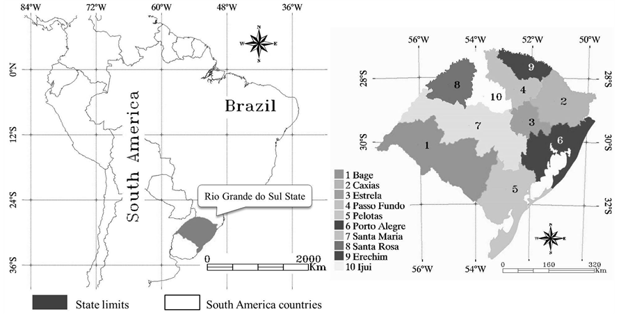
Figure 1. Rio Grande do Sul State and regional study areas from EMATER.
Three droughts occurred in the study period, which severely affected the summer crops of 2004, 2005 and 2012. The most severe drought in 2005 caused a 75% loss of the soybean production [18] when the temperature averages over the crop canopy were approximately 7 K higher than the ideal conditions [24] .
Typically, RS is rain-fed, and the irrigation systems designed for soybean crop areas cover only 170,000 ha [42] [43] , which comprised less than 4.5% of the total soybean areas in the state in 2006 [18] .
2.2. Crop Area Analysis
The soybean crop areas have been identified by application of the MCDA (MODIS Crop Detection Algorithm), which was developed for crop area estimation and is fully described by [29] . A crop area map for ten different crop years was generated from a map composition that combines each crop year map from 2003 to 2012. The resulting crop area map composition tagged all soybean crop pixels at a frequency equal to or greater than two events, which totalled 5.37 million hectares. Figure 2 shows the resulting soybean map using the MCDA procedure.
2.3. Data Type and Resolution
Several sources of data were used in this study: 1) annual soybean agricultural statistics at the state and municipality levels [23] for the entire study area were used to compare and evaluate the results obtained from our soybean area estimation procedure; 2) soybean cropping calendars were provided by the State Agency EMATER (Associação Riograndense de Empreendimentos de Assistência Técnica de Extensão Rural) for the crop years of 2003, 2004 and 2005; 3) LST data from 2003 to 2012 derived from the MODIS sensor on board the Aqua satellite (product MYD11A2-collection 5) were used to derive temperatures over the soybean canopy (canopy-LST) in the crop years between 2003 and 2012. This product was preferred because it is obtained during the afternoon passage. Collection 5 products hada mean and standard deviation of the LST differences of less than 0.2 K and 0.5 K, respectively [44] ; 4) official data reports and historical statistics of soybean crop production from IBGE were obtained; 5) official data reports and historical statistical data of soybean crop areas from IBGE were used to calculate soybean yields over the entire study area; 6) Enhanced Vegetation Index (EVI) data from 2003 to 2012 derived from the MODIS sensor on board the Terra satellite (product MOD13Q1-collection 5), which is composed of the best radiometric and geometric pixels selected within a 16-day period, were used to classify the canopy-LST as an auxiliary data because the vegetation index and LST interpret opposite extreme weather events [45] . The EVI data are representative of vegetation vigour. EVI is based on canopy reflectance characteristics and is designed to minimise the influence of soil and atmospheric effects on satellites [46] [47] .
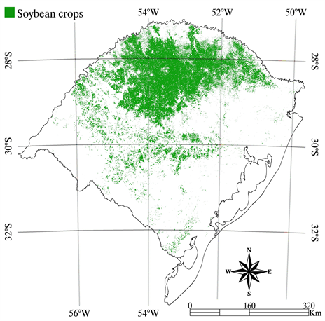
Figure 2. Soybean crop area map composition for crop years 2003 to 2012.
The EVI expression is 2.5*(Nir − Red)/(Nir + 6 Red − 7.5 Blue + 1), where Nir, Red and Blue are atmospherically or partially atmospherically corrected surface reflectance of near infrared, red and blue bands, respectively [46] . The MODIS images and products were pre-processed by the National Aeronautics and Space Administration [48] and are available at no charge at https://lpdaac.usgs.gov/data_access/data_pool.
2.4. Vegetation Development
Agricultural crop production is characterised by a large variability in yield as a result of the main agrometeorological parameters [25] . This is particularly evident in Rio Grande do Sul State, where agrometeorological conditions during the summer are known to vary spatially and annually causing different impacts on yield.
Recently, yield estimation models have considered agricultural practices, weather or climatological conditions as the predominant physically driven conditions that represent the cycle of agricultural development [24] , especially precipitation [20] [21] [26] . In RS State, [27] calculated the relationship between soybean yields and vegetation vigour from EVI; they obtained an R2 = 0.91 for a municipality level analysis by considering an integrative window of the soybean crop cycle. However, agriculture is also impacted by crop canopy temperature extremes, such as heat waves [17] [24] [49] . Figure 3 presents the high variability of yield in RS.
The preferred period of soybean sowing in RS is from mid-October to mid-December, according to agricultural zoning for lower climatic risk within various soils, regions and cultivars [50] . Depending on the sowing date, maximum plant growth is observed from late January to early March [29] . The flowering period is typically reached between late January and early March (EMATER), as observed during the 2003 to 2005 period. Figure 4 present the mean agricultural calendar for soybean in RS.
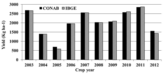
Figure 3. Soybean yield averages in Rio Grande do Sul State from 2003 to 2012.
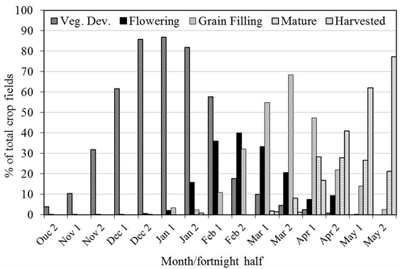
Figure 4. Average agricultural calendar for soybean crops in Rio Grande do Sul, from EMATER-RS (2003-2005).
2.5. Canopy-LST and Soybean Crop Yield
LST is a measure of surface temperature (also known as skin temperature), rather than air temperature, which is more commonly applied in physiological studies [51] . The theoretical basis is Planck’s Law of Radiation, which describes that radiating energy from a black-body, as predict by Stefan-Boltzmann’s Law, is distributed in the electromagnetic spectrum as a function of its temperature [52] . Thus, the LST is the internal manifestation of the random translational energy of the molecules constituting a body [53] [54] . Several applications of thermal radiation have used the black-body radiation theory for temperature estimations since the pioneer studies of Dick, Penzias and Wilson in the 1950s [54] . For Earth Science studies, the external manifestation of an object’s energy can be detected by remotely sensed devices into an orbital path way using thermal scanning technology [55] . Therefore, it is possible to obtain a physical measure from the vegetation that covers the surface.
Considering that physiological activities of leaves are closely related to their actual temperature (canopy temperature), rather than air temperature, the LST can be used as a reliable measure of physiological activity of a vegetation canopy [51] [56] , because the vegetation structures of soybeans with planophile canopies are prone to preserve spectral emissivity information [57] . Canopy-LST can exert a direct effect on plant photosynthesis. Among the main impacts of heat stress, the effect on photosynthesis is the most important on yields due to the inhibition of the crop growth rate [17] . Canopy temperatures between 298 K (25˚C) and 309 K (35˚C), with an ideal average near 303 K (30˚C), are most frequently considered the ideal conditions for soybean development [14] [17] [35] . Nevertheless, studies have demonstrated that the combined use of the LST and vegetation index assumes an inverse mathematical relationship [24] [36] [58] .
2.6. Satellite Data Retrieval and Processing
To generate the yield map, spatially interpolated maps were obtained using the spherical/ordinary kriging method, which is based on the trend of the variability in the sample’s values and the distance between them [59]. This technique is adequate for the conditions identified in the present study, where a limited number of meteorological stations were available. To generate spatially interpolated maps, average yield values for each municipality were placed at their centroids. Then they were defined at the regional scale to generate regional averages of yield, EVI and accumulated rainfall.
First, we acquired MODIS/Terra data (MOD13Q1 product-collections 5) and MODIS/Aqua data (MYD11A2) that covered the entire RS State (image tiles: H13V11 and H13V12) for the 2003-2012 study period. The 496 municipalities were grouped into ten regional areas of EMATER. It is important to note that the analysis of deviations from the smoothed maps was only performed on the areas mapped as soy cultivation between 2003 and 2012. The original LST data product (MYD11A2), as distributed by NASA, corresponds to composites of eightday averages. The original vegetation index product (MOD13Q1) is distributed for 16-day maximum value composites. Thus, to match the LST product to the EVI product, we rearranged data and grouped them as follows:
1) MOD13Q1 already represents a maximum composite of 16 days; thus, any further calculation was performed within 16 days of EVI, starting from DOY 001;
2) To retrieve the most representative LST data from the crop canopy, the first step was to obtain the maximum LST composition over 16 days by combining two MYD11A2 products (an average of eight days) that cover the same DOY period from item 1;
3) After that, steps 1 and 2 were also performed for the subsequent 16-day composites of MYD11A2 and MOD13Q1;
4) By combining two LST composites of 16 days as a function of the maximum EVI, the canopy-LST composite of 32 days is obtained. Therefore, the resulting product at DOY 001 is representative of the temperatures over crop canopies that occurred when the EVI was maximum between DOY 001 and 032. Canopy-LST at DOY 017 is representative of the temperatures over crop canopies that occurred when the EVI was maximum between DOY 017 and 056, and so on. An earlier analysis of canopy-LST (prior to DOY 001) was not performed due to the heterogeneous surface, which characterises the initial phenological stage. Such conditions can induce spatial variations of several degrees in the near surface air temperature [60] and consequently in the canopy-LST because of the absence of the soybean vegetation canopy in the initial development period;
5) Canopy-LST maps are generated for different time periods of the phenological stage, which cover a time window of 32 days (DOY 001; 017; 033; 049) (as presented in Figure 5(b)). All Canopy-LST maps and Yield
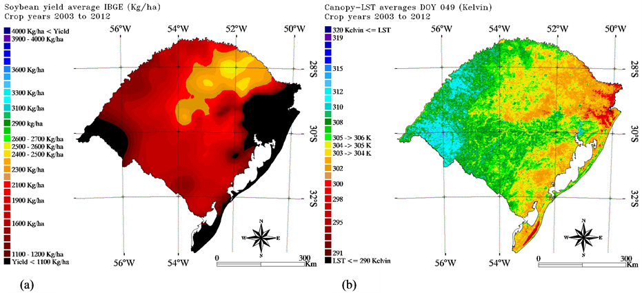
Figure 5. Distribution of the yield average (a) obtained between 2003 and 2012 and (b) canopy-LST map in DOY 049.
map were merged with the crop area map from MCDA;
6) Finally, the percentage variation of each regional average canopy-LST composite was compared to its average from 2003 to 2012 in the same time window. This calculation is performed such that the generated LST is associated with the maximum EVI that occurs in one of the two 16-day composites. The detailed procedure is important because we are not interested in the maximum LST registered in the time window of 32 days, but rather we were valuing the LST associated with the best vegetation coverage of the time window, which is considered the canopy-LST in order to avoid a previous moisture background and/or drought effects. Here we note that the concept of the former mentioned calculation is completely different from the latter.
Although studies of crop modelling that use LST data very often do not adequately adhere to these fundamentals, for cold or heat effects on vegetation, the physical concepts in the previously mentioned review sections must be seriously considered before processing the imagery.
3. Results
Soybean yields in RS State obtained from IBGE were compared to the canopy-LST at various development stages at the state and regional scales from 2003 to 2012. Spatially interpolated maps of the yield average distribution (Figure 5(a)) and the canopy-LST distribution for DOY 001, 017, 033, 049 and 065 (Figure 5(b)) were obtained. Linear least square regression analysis was performed for state level soybean production estimates that were obtained from IBGE for the same period. A LST analysis was performed on the Kelvin scale; therefore, each 1% percent deviation from the average corresponds to approximately 3 K. Figure 6 presents the relative yield distribution as a function of the relative canopy-LST in RS.
The soybean yield deviations from each crop year were compared to the canopy-LST deviation. An analysis of the data shows a well-defined trend for higher yields and below average canopy-LST occurrences and lower yields for above average LST (Figures 6(c) and (d)).
To better understand the canopy-LST impacts and its correlation to yields, all of the data were analysed as deviations from the averages between 2003 and 2012. Through a non-linear relationship, it was observed that variations in the canopy-LST averages from DOY 033 (between February 2nd and March 5th), which is fully related to the flowering period in Figure 4 (Feb. 1-Feb. 2), are characterised by R2 = 0.68 and RMSD = 19.3%. However, a linear relationship with R2 = 0.82 and RMSD = 14.4% is obtained at DOY 049 (between February 18th and March 21st), which is more closely related to the grain filling period (Feb. 2-Mar. 1).
The dense group of points placed in the inferior right quadrant of Figure 6(f) represent points with a relative canopy-LST above 2% in all ten regions in the summer crop year of 2005. As observed by [24] , these higher canopy-LST deviations in 2005 are linked to the most severe drought occurrence of the study period. Considering a minimum yield of 1000 kg∙ha−1, the overall yield average inside the crop areas from 2003 to 2012 was
 (a) (b)
 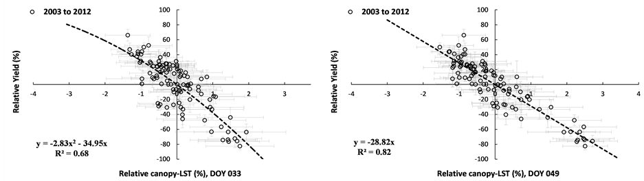 (c)(d)
 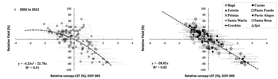 (e)(f)
Figure 6. Scatter grams that compare the relative yield distribution as a function of the relative canopy-LST obtained from crop years 2003 to 2012.
2003 kg∙ha−1 with a standard deviation of 308 kg∙ha−1. Considering DOY 049, the overall average canopy-LST is 305.0 K (31.8˚C) with a standard deviation of 1.9 K, the minimum is 296.4 K (23.2˚C), and the maximum is 315.0 K (41.8˚C). These physically driven conditions led to a linear decreasing relationship of −28.7%. However, when considering drought-free crop years (without 2005 and 2012), the new overall yield average is 2260 kg∙ha−1 with a standard deviation of 326 kg∙ha−1. Under these conditions, the new overall average canopy-LST is 303.6 (30.4˚C) with a standard deviation of 1.8 K, the minimum is 295.8 (22.6˚C), and the maximum is 313.0 K (39.8˚C), which are close to the suggested limit of the ideal temperature conditions.
4. Discussion
The heat stress that occurs during flowering and pod formation (R1-R5) affects grain numbers, which is closely related to the yield [35] [38] where as stress during grain filling (R5-R7) reduces the grain size [38] . When energy and water conditions are non-limiting for plant growth, considering complete canopy conditions, crops can present elevated canopy-LST due to aerodynamic resistances that suppress sensible heat transfer [32] . When evaluated cotton plant (C3 plant as soybean) development under stress conditions and [10] observed that the direct effects of temperature on reproductive processes (flowering) are difficult to distinguish from metabolic processes because the inhibition of photosynthesis can also be caused by overheating the canopy, even under well-watered conditions. However, in the present investigation, considering the drought-induced crop years of 2005 and 2012 (Figures 3 and 6(f)), yield loss may be associated with the coupled effect of two different physically driven conditions: an initial reduction in the water availability followed by a temperature increase, which is probably exacerbated by the energy exchange mainly due to wind, humidity and exposure to incident radiation [32] [61] [62] .
As presented in Figure 4, the average agricultural calendar for ten different regions in the state presents three maxima of the flowering period from the first half of February to the first half of March that are greater than 30%. Although DOY 049 also covers the flowering period, similar to DOY 033, we note that the results for DOY 049 are more correlated. However, this result is possibly linked to the computational redundancy of the canopy-LST data to yield losses due to drought. As the canopy-LST in the DOY 049 window covers the last end of the crop development profile, the damaging effects due to heat waves may overlap with early drought effects that may have begun several weeks prior, especially for crop years 2005 and 2012. In this situation, the implementation of strategies and policy planning for the region, such as a sowing calendar and the use of irrigation techniques [22] , are extremely important. Heat waves can potentially increase drought effects by overheating the vegetation canopy, which inhibits photosynthesis [10] [63] and intensifies plant damage (Figure 6(f)). Furthermore, it is important to note that, considering the mean agriculture calendar (Figure 4), DOY049 does not correlate as well as DOY 033 with the flowering period (Figure 6(c)), but it does correlate better to grain filling (Figure 6(f)). This suggests that, although higher temperatures can occur in the earlier phenological stages (as during flowering), severe impacts on yields are prone to be observed during the grain filling stage, especially when the elevated canopy-LST is associated with drought(e.g., crop years 2005 and 2012) (Figure 3).
The relatively smaller correlations between canopy-LST and yield for the 32-day composite windows presented in Figures 6(a) and (b) can be linked to background effects. The periods covered are DOY 001 between January 1st and February 1st (Jan 1-Jan 2 in Figure 4) and DOY 017 between January 17th and February 17th (Jan 2-Feb 1 in Figure 4). Soil cover by vegetation during this stage is sparse, which increases surface temperature and may be confused with an unrealistic rise in the canopy-LST.
5. Conclusions
We observed that variations of the averages of canopy-LST during flowering/grain filling periods of summer crops are closely associated with variations in soybean yields.
The results indicate that heat waves that are slightly warmer than the optimal conditions for growth can potentially increase drought effects and yield loss by overheating the vegetation canopy and intensifying plant damage.
Finally, we concluded that future studies on canopy-LST monitoring can significantly contribute to the regional characterisation of agriculture vulnerability and management of potential climate conditions and fluctuations.
Acknowledgements
We wish to thank Vale do Rio dos Sinos University (UNISINOS). Additionally, we thank the National Aeronautical and Space Administration (NASA) for the Terra and Aqua/MODIS data. We especially thank the Conselho Nacional de Desenvolvimento Científico e Tecnológico (CNPq) for their support.
References
- UNEP—United Nations Environment Programme (2009) Environmental Food Crisis. The Environment’s Role in Averting Future Food Crises. http://www.unep.org/pdf/foodcrisis_lores.pdf
- Masuda, T. and Goldsmith, P.D. (2009) World Soybean Production: Area Harvested, Yield, and Long-Term Projections. International Food and Agribusiness Management Review, 12, 143-163.
- Lobell, D.B., Burke, M.B., Tebaldi, C., Mastrandrea, M.D., Falcon, W.P. and Naylor, R.L. (2008) Prioritizing Climate Change Adaptation Needs for Food Security in 2030. Science, 319, 607-610. http://dx.doi.org/10.1126/science.1152339
- Batistti, D.S. and Naylor, R.L. (2009) Historical Warnings of Future Food Insecurity with Unprecedented Seasonal Heat. Science, 323, 240-244. http://dx.doi.org/10.1126/science.1164363
- Streck, N.A. and Alberto, C.N. (2006) Estudo numérico do impacto da mudança climática sobre o rendimento de trigo, soja e milho. Pesquisa Agropecuária Brasileira, 41, 1351-1359. http://dx.doi.org/10.1590/S0100-204X2006000900002
- FAO—Food and Agriculture Organization (2011) The State of Food Insecurity in the World.http://www.fao.org/docrep/013/i2050e/i2050e07.pdf
- Meehl, G.A., Stocker, T.F., Collins, W.D., Friedlingstein, P., Gaye, A.T., Gregory, J.M., Kitoh, A., Knutti, R., Murphy, J.M., Noda, A., Raper, S.C.B., Watterson, I.G., Weaver, A.J. and Zhao, Z.-C. (2007) Global Climate Projections. In: Solomon, S., Qin, D., Manning, M., Chen, Z., Marquis, M., Averyt, K.B., Tignor, M. and Miller, H.L., Eds., Climate Change 2007: The Physical Science Basis. Contribution of Working Group I to the Fourth Assessment Report of the Intergovernmental Panel on Climate Change, Cambridge University Press, Cambridge and New York, 747-846.
- Gorman, P.A. and Schneider, T. (2009) The Physical Basis for Increases in Precipitation Extremes in Simulations of 21st-Century Climate Change. Proceedings of the National Academy of Sciences, 106, 14773-14777.http://dx.doi.org/10.1073/pnas.0907610106
- Rosenzweig, C., Iglesius, A., Yang, X.B., Epstein, P. and Chivian, E. (2001) Climate Change and Extreme Weather Events: Implications for Food Production, Plant Diseases, and Pests. NASA Publications-Paper 24, 2, 90-104.
- Carmo-Silva, A.E., Gore, M.A., Andrade-Sanchez, P., French, A.N., Hunsaker, D.J. and Salvucci, M.E. (2012) Decreased CO2 Availability and Inactivation of Rubisco Limit Photosynthesis in Cotton Plants under Heat and Drought Stress in the Field. Environmental and Experimental Botany, 83, 1-11. http://dx.doi.org/10.1016/j.envexpbot.2012.04.001
- Howden, S.M., Soussana, J.-F., Tubiello, F.N., Chhetri, N. Dunlop, M. and Meinke, H. (2007) Adapting Agriculture to Climate Change. Proceedings of the National Academy of Sciences, 104, 19691-19696.
- Wheeler, T.R., Craufurd, P.Q., Ellis, R.H., Porter, J.R. and Prasad, P.V.V. (2000) Temperature Variability and the Yield of Annual Crops. Agriculture, Ecosystems and Environment, 82, 159-167.http://dx.doi.org/10.1016/S0167-8809(00)00224-3
- Sediyama, T. (2009) Tecnologias de produção e usos da soja. Mecenas, Londrina, 314.
- Khan, A.Z., Shah, P. Khan, H., Nigar, S., Perveen, S., Shah, M.K., Amanullah, A., Khalil, S.K., Munir, S. and Zubair, M. (2011) Seed Quality and Vigor of Soybean Cultivars as Influenced by Canopy Temperature. Pakistan Journal of Botany, 43, 643-648.
- Lobell, D.B. and Asner, G.P. (2003) Climate and Management Contributions to Recent Trends in US Agricultural Yields. Science, 229, 1032. http://dx.doi.org/10.1126/science.1077838
- Meerburg, B.G., Verhagen, A., Jongschaap, R.E.E., Franke, A.C., Schaap, B.F., Dueck, T.A. and van der Werf, A. (2009) Do Nonlinear Temperature Effects Indicate Severe Damages to US Crop Yields under Climate Change? Proceedings of the National Academy of Sciences, 106, 120. http://dx.doi.org/10.1073/pnas.0910618106
- Schlenker, W. and Roberts, M. (2009) Nonlinear Temperature Effects Indicate Severe Damages to US Crop Yields under Climate Change. Proceedings of the National Academy of Sciences, 106, 15594-15598.http://dx.doi.org/10.1073/pnas.0906865106
- CONAB—Companhia Nacional de Abastecimento (2012) Acompanhamento da safra brasileira de grãos. CONAB/ DIPAI/SUINF/GEASA. Conab: Brasília. http://www.conab.gov.br/OlalaCMS/uploads/arquivos/12_09_06_09_18_33_boletim_graos_-_setembro_2012.pdf
- Matzenauer, R., Barni, N.A. and Maluf, J.R.T. (2003) Estimative of the Relative Water Consumption of Soybean in Rio Grande do Sul State, Brazil. Ciência Rural, 33, 1013-1019.http://dx.doi.org/10.1590/S0103-84782003000600004
- Fontana, D.C., Weber, E., Ducati, J.R., Berlato, M.A., Guasselli, L.A. and Gusso, A. (2002) Monitoramento da cultura da soja no centro—Sul do Brasil durante La Niña de 1998/2000. Revista Brasileira de Agrometeorologia, 10, 343-351.
- Ferreira, D.B. (2010) Análise da variabilidade climática e suas consequencias para a produtividade da soja na região sul do Brasil. Ph.D. Thesis, INPE, São José dos Campos.
- Melo, R.W., Fontana, D.C. and Berlato, M.A. (2004) Indicadores de produção de soja no Rio Grande do Sul comparados ao zoneamento agrícola. Pesquisa Agropecuária Brasileira, 39, 1167-1175. http://dx.doi.org/10.1590/S0100-204X2004001200002
- IBGE—Instituto Brasileiro de Geografia e Estatística (2012) SIDRA: Sistema IBGE de recuperação automática. http://www.sidra.ibge.gov.br/
- Gusso, A. (2013) Integration of NOAA/AVHRR Images: Cooperation Network towards National Soybean Crop Monitoring. Revista Ceres, 60, 43-52.
- Esquerdo, J.C.D.M., Zullo, J. and Antunes, J.F.G. (2011) Use of NDVI/AVHRR Time-Series Profiles for Soybean Crop Monitoring in Brazil. International Journal of Remote Sensing, 32, 3711-3727. http://dx.doi.org/10.1080/01431161003764112
- De Melo, R.W., Fontana, D.C., Berlato, M.A. and Ducati, J.R. (2008) Anagrometeorological-Spectral Model to Estimate Soybean Yield, Applied to Southern Brazil. International Journal of Remote Sensing, 29, 4013-4028. http://dx.doi.org/10.1080/01431160701881905
- Gusso, A., Ducati, J.R., Veronez, M.R., Arvor, D. and Silveira Jr., L.G. (2013) Spectral Model for Soybean Yield Estimate Using MODIS/EVI Data. International Journal of Geosciences, 4, 1233-1241.http://dx.doi.org/10.4236/ijg.2013.49117
- Junges, A.H., Fontana, D.C. and Melo, R.W. (2012) Caracterização do cultivo de trigo na região norte do Estado do Rio Grande do Sul através das estimativas oficiais de área cultivada, produção e rendimento de grãos. Ciência Rural, 42, 31-37. http://dx.doi.org/10.1590/S0103-84782011005000153
- Gusso, A., Adami, M., Formaggio, A.R., Rizzi, R. and Rudorff, B.T.F. (2012) Soybean Area Estimation and Mapping by Means MODIS/EVI Data. Pesquisa Agropecuária Brasileira, 47, 425-435.http://dx.doi.org/10.1590/S0100-204X2012000300015
- Mabilana, H.A., Fontana, D.C. and Fonseca, E.L. (2012) Desenvolvimento de modelo agrometeorológico espectral para estimativa de rendimento do milho na Província de Manica-Moçambique. Revista Ceres, 59, 337-349.http://dx.doi.org/10.1590/S0034-737X2012000300007
- Seiler, R.A., Kogan, F. and Sullivan, J. (1998) AVHRR-Based Vegetation and Temperature Condition Indices for Drought Detection in Argentina. Advances in Space Research, 21, 481-484. http://dx.doi.org/10.1016/S0273-1177(97)00884-3
- Nemani, R. and Running, S. (1997) Land Cover Characterization Using Multitemporal Red, Near-Ir and Thermal-Ir Data from NOAA/AVHRR. Ecological Applications, 7, 79-90. http://dx.doi.org/10.1890/1051-0761(1997)007[0079:LCCUMR]2.0.CO;2
- Running, S.W., Loveland, T.R., Pierce, L.L., Nemani, R.R. and Hunt, E.R. (1995) A Remote Sensing Based Vegetation Classification Logic for Global Land Cover Analysis. Remote Sensing of Environment, 51, 39-48. http://dx.doi.org/10.1016/0034-4257(94)00063-S
- Liu, W.T. and Kogan, F. (2002) Monitoring Brazilian Soybean Production Using NOAA/AVHRR Based Vegetation Indices. International Journal of Remote Sensing, 23, 1161-1179. http://dx.doi.org/10.1080/01431160110076126
- Board, J.E. and Kahlon, C.S. (2007) Soybean Yield Formation: What Controls It and How It Can Be Improved. In: El-Shemy, H.A., Ed., Soybean Physiology and Biochemistry, InTech Open Access, Rijeka, 1-36.
- Hope, A.S., Petzold, D.E., Goward, S.N. and Ragan, R.M. (1986) Simulated Relationships between Spectral Reflectance Thermal Emissions and Evapotranspiration of a Soybean Canopy. Journal of the American Water Resources Association, 22, 1011-1019. http://dx.doi.org/10.1111/j.1752-1688.1986.tb00772.x
- Rodrigues, O., Didonet, A.D., Lhamby, J.C.D., Bertagnolli, P.F. and Luz, J.S. (2001) Resposta quantitativa do florescimento da soja à temperatura e ao fotoperíodo. Pesquisa Agropecuária Brasileira, 36, 431-437. http://dx.doi.org/10.1590/S0100-204X2001000300006
- Gibson, L.R. and Mullen, R.E. (1996) Soybean Seed Quality Reductions by High Day and Night Temperature. Crop Science, 36, 1615-1619. http://dx.doi.org/10.2135/cropsci1996.0011183X003600060034x
- Craufurd, P.Q. and Wheeler, T.R. (2009) Climate Change and the Flowering Time of Annual Crops. Journal of Experimental Botany, 60, 2529-2539. http://dx.doi.org/10.1093/jxb/erp196
- Koppen, W. (1948) Climatologia. Fondo de Cultura Economica, Mexico, 71.
- INMET—Instituto Nacional de Meteorologia (2009) Normais Climatológicas do Brasil de 1961 a 1990. http://www.inmet.gov.br/portal/index.php?r=bdm ep/bdmep
- Saraiva, K.R. and Souza, F. (2012) Estatísticas sobre irrigação nas regiões sul e sudeste do Brasil segundo o censo agropecuário 2005-2006. Revista Irriga, 17, 168-176.
- Paulino, J., Folegatti, M.V., Zolin, C.A., Sánchez-Román, R.M. and José, J.V. (2011) Situação da agricultura irrigada no Brasil de acordo com o censo agropecuário 2006. Revista Irriga, 16, 163-176.
- Wan, Z.M. (2008) New Refinements and Validation of the MODIS Land-Surface Temperature/Emissivity Products. Remote Sensing of Environment, 112, 59-74. http://dx.doi.org/10.1016/j.rse.2006.06.026
- Seiler, R.A. and Kogan, F. (2002) Monitoring ENSO Cycles and Their Impacts on Crops in Argentina from NOAA-AVHRR Satellite Data. Advances in Space Research, 30, 2489-2493. http://dx.doi.org/10.1016/S0273-1177(02)80316-7
- Huete, A., Didan, K., Miura, T., Rodriguez, E.P., Gao, X. and Ferreira, L.G. (2002) Overview of the Radiometric and Biophysical Performance of the MODIS Vegetation Indices. Remote Sensing of Environment, 83, 195-213. http://dx.doi.org/10.1016/S0034-4257(02)00096-2
- Justice, C.O., Townshend, J.R.G., Vermote, E.F., Masuoka, E., Wolfe, R.E., Saleous, N., Roy, D.P. and Morisette, J.T. (2002) An Overview of MODIS Land Data Processing and Product Status. Remote Sensing of Environment, 83, 3-15. http://dx.doi.org/10.1016/S0034-4257(02)00084-6
- NASA-National Aeronautics and Space Administration (2014) Land Processes Distributed Active Archive Center (LPDAAC). https://lpdaac.usgs.gov/data_access/data_pool
- Kogan, F. (2001) Operational Space Technology for Global Vegetation Assessment. Bulletin of the American Meteorological Society, 82, 1949-1964. http://dx.doi.org/10.1175/1520-0477(2001)082<1949:OSTFGV>2.3.CO;2
- Cunha, G.R., Barni, N.A., Haas, J.C., Maluf, J.R.T., Matzenauer, R., Pasinato, A., Pimentel, M.B.M. and Pires, J.L.F. (2001) Zoneamento agrícola e época de semeadura para soja no Rio Grande do Sul. Revista Brasileira de Agrometeorologia, 9, 446-459.
- Sims, D.A., Rahman, A.F., Cordova, V.D., El-Masri, B.Z., Baldocchi, D.D, Bolstad, P.V., Flanagan, L.B., Goldstein, A.H., Hollinger, D.Y., Misson, L., Monson, R.K., Oechel, W.C., Schmid, H.P., Wofsy, S.C. and Xu, L. (2008) A New Model of Gross Primary Productivity for North American Ecosystems Based Solely on the Enhanced Vegetation Index and Land Surface Temperature from MODIS. Remote Sensing of Environment, 112, 1633-1646. http://dx.doi.org/10.1016/j.rse.2007.08.004
- Hecht, E. (1998) Optics. 3rd Edition, Addison-Wesley, Reading, 694.
- Lillesand, T.M., Kiefer, R.W. and Chipman, J.W. (2003) Remote Sensing and Image Interpretation. 5th Edition, John Wiley & Sons, Hoboken.
- Eisberg, R. and Resnik, R. (1985) Quantum Physics of Atoms, Molecules, Solids, Nuclei and Particles. 2nd Edition, Wiley, Hoboken, 928.
- Elachi, C. (1987) Introduction to the Physics and Techniques of Remote Sensing. Wiley, New York.
- Diak, G.R. and Whipple, M.S. (1993) Improvements to Models and Methods for Evaluating the Land-Surface Energy Balance and Effective Roughness Using Radiosonde Reports and Satellite-Measured Skin Temperature Data. Agricultural and Forest Meteorology, 63, 189-218. http://dx.doi.org/10.1016/0168-1923(93)90060-U
- Salisbury, J.W. (1986) Preliminary Measurements of Leaf Spectral Reflectance in the 8-14 um Region. International Journal of Remote Sensing, 7, 1879-1886. http://dx.doi.org/10.1080/01431168608948981
- Sandholt, L., Rasmunssen, K. and Andersen, J. (2002) A Simple Interpretation of the Surface Temperature/Vegetation Index Space for Assessment of Surface Moisture Status. Remote Sensing of Environment, 79, 213-224. http://dx.doi.org/10.1016/S0034-4257(01)00274-7
- Jian-Guo, L. and Mason, P.J. (2009) Essential Image Processing and GIS for Remote Sensing. Wiley-Blackwell, 460.
- Anderson, M.C., Norman, J.M., Diak, G.R., Kustas, W.P. and Mecikalski, J.R. (1997) A Two-Source Time-Integrated Model for Estimating Surface Fluxes Using Thermal Infrared Remote Sensing. Remote Sensing of Environment, 60, 195-216. http://dx.doi.org/10.1016/S0034-4257(96)00215-5
- Wan, Z., Wang, P. and Li, X. (2004) Using MODIS Land Surface Temperature and Normalized Difference Vegetation Index Products for Monitoring Drought in the Southern Great Plains, USA. International Journal of Remote Sensing, 25, 61-72. http://dx.doi.org/10.1080/0143116031000115328
- Peterson, T.C., Stott, P.A. and Herring, S. (2012) Explaining Extreme Events of 2011 from a Climate Perspective. American Meteorological Society, 93, 1041-1067.
- Salvucci, M.E. (2008) Association of Rubisco Activase with Chaperonin-60β: A Possible Mechanism for Protecting Photosynthesis during Heat Stress. Journal of Experimental Botany, 59, 1923-1933. http://dx.doi.org/10.1093/jxb/erm343
NOTES

*Measurements are inclusive of drought and heat wave effects.
#Corresponding author.